In this lab, we will inject an audio signal into the FPGA using the XADC block to digitize. The signal can be put into a FIFO for readout by the RPi, to do signal processing analysis. In addition, we will implement an auto-correlator inside the FPGA that will allow the RPi to look at integrated signals. This project will be built on what we did in the previous Increasing Bandwidth project.

To start, open the "BLAST" project and save as a new project, which we will call "AUDIO". We will be building from that project.

Digitizing audio signals

Audio signals are traditionally digitized with a sampling rate of 44.1kSps. This value was set back in the days when CD's were being developed. During those early days of music as data, hard drives did not have enough memory to store a full CD worth of data which was originally around 700MBytes. So when creating the digital data during recording, engineers used video recorders to store the digital data from the sampling. In the US, these video recorders ran at 30 frames/sec and allowed 490 usable lines per frame for video. So a decision was made to store 3 audio samples per line of video, so 3×30×490=44100, hence the sampling rate of 44.1kHz has stuck with us ever since. In this project, we will use the XADC to digitize the incoming audio voltage at 44.1kHz, just like we did in the Increasing Bandwidth project. We could actually use any sampling we like, but let's stick with the standard so that the RPi could in principle save the data into an mp3 format if that's what you want to do.

The code for top.v will be exactly the same as in the previous project, and should be all set when you clone AUDIO from BLAST.

We will start with no changes to AUDIO, and inject an AC sinusoidal voltage into the FPGA using the same VAUX6P/N inputs as in previous project. Remember, the XADC we have configured is unipolar, so you have to take care to inject an AC signal with a DC offset so that you can see the entire waveform. For what's below, I used an old Wavetek Sweep Generator (model 184) that you can get on eBay for probably $50.

RPi Python code

Let's start with blast.py and add detailed capability to be able to read and write the Control and Blast registers, and to read the Status register and display. The modifications that accomplish this can be found here. When you run this on the RPi, you should see the following:

Hit the "BLAST!" button, it should take around 5 seconds to collect all the data into the RPi. Then hit the "Plot" button, which implements the matplotlib plotting via the following simple code:

    plt.plot(self.voltages)
    plt.show()

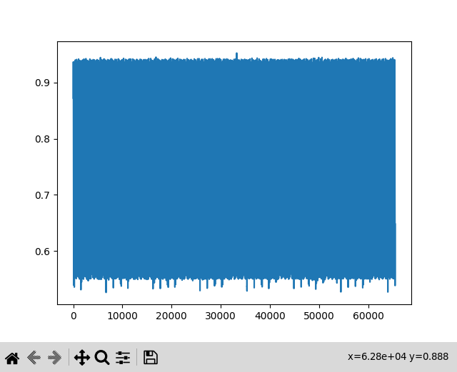
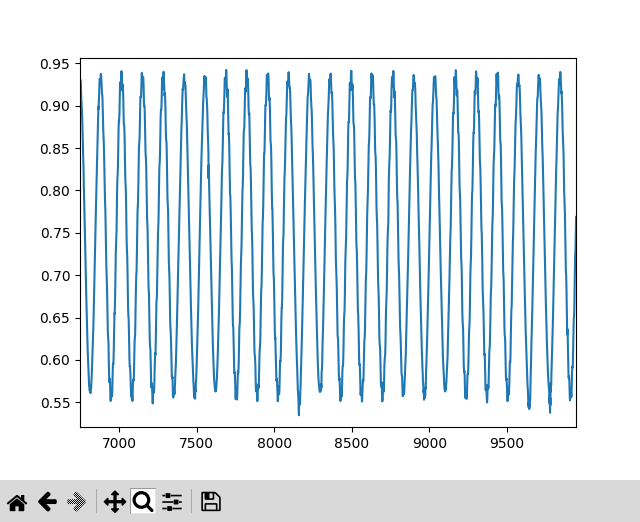
The signal input is oscillating at around 320Hz, which means it has a period of around 3ms. If we are digitizing at 44.1kHz, then the time between digitizations will be 22.67μs, so the waveform will repeat every 44100/320 = ~137 points. There are almost 35535 points in the plot above, so we are looking at 260 periods of our oscillating wave, which is why what you see looks like a solid figure. Click on the magnifying glass and select a small portion of the horizontal range and the full vertical, and you should see this:

We should check the frequency using a FFT calculation that Python can provide easily via the following code:

    def fourierAll(self):
        #
        #   I suppose python can do this better, but when I tried, I
        #   got nonsensical results so I'm doing it myself.  what the hell
        #
        amp = []
        f0 = 44100.0    # incoming frequency
        N = 2000 #or set to len(self.voltages)
        test = False
        fake = []
        if test:
            print("using fake data: ")
            for i in range(0,N):
                x = 0.5 + 0.4*math.sin(2*math.pi*i/88)
                fake.append(x)
                #print(str(x))
        omega = 2.0*math.pi/N
        npts = len(self.voltages)   # use all points
#       npts = 1000  # you can change this if you like
        #
        #   don't worry about n=0, the DC offset
        #
        yf = np.fft.rfft(self.voltages)
        freq = np.fft.rfftfreq(len(self.voltages),1./f0)
        plt.plot(freq,np.abs(yf))
        plt.show()

This is invoked by hitting the "Fourier" button. It will pop up a window that shows this:

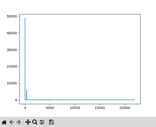
Here you see the huge DC offset followed closely by another smaller peak. If you zoom in on the peak, you should see the following:

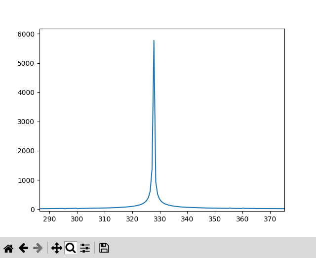
This is what we expect from a monochromatic input at around 328Hz.

Audio Signals

To get real audio into the FPGA from sound, we need a microphone with some kind of amplifier. I found a very nice gadget on adafruit.com that costs $8:

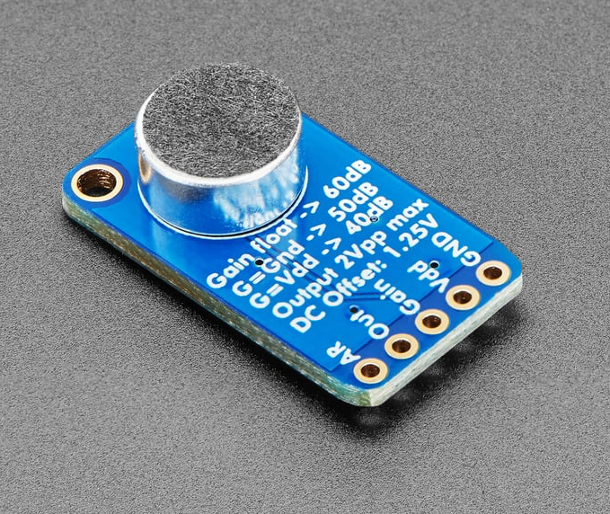
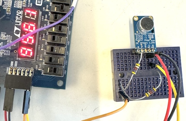
It can be found here. The microphone range is 20-20kHz, and the amplifier has a variable gain (40, 50, and 60db that you select by jumpering) with a maximum output amplitude of 1V (2Vpp) on a 1.25V DC bias, which we need to get rid of. Or, instead of eliminating it with a blocking capacitor and a DC offset, we just divide the signal down by a factor of 1/3 so that the DC bias is closer to 0.5V, and if the amplitude is not to great, it should appear nicely inside our 0-1 range of the XADC. As you can see in the diagram below, we power the Electret gadget using the 3.3V and ground from the FPGA (red and black wires), then take the output and place a 15kΩ and a 5kΩ resistor to ground. The voltage input to the XADC will be across the lower 5kΩ resistor, giving us a 1/3 divider (orange wire to the positive input of the XADC, yellow to the negative).

The amplifier has several gains. Default gain is 60dB, which is fine but you will need the input sound to be rather close to the microphone or it will be way down in the noise. To see how well this works, we can use a waveform generator app on the iPhone to generate a 500Hz square wave, input to the microphone, and capture the waveform in the FIFO and look at the frequency spectrum as seen in the figure below. You can also run with a 40dB and 50dB gain by jumpering the "Gain" pin to either VCC or ground respectively (it's printed on the circuit board.)

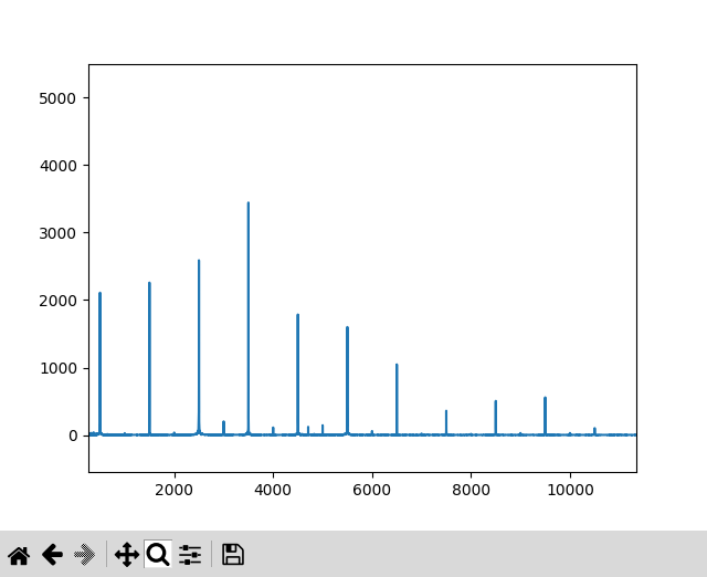
The fundamental on the left is at 500Hz, and you can see the various overtones. Why there are overtones that appear to be half integer multiples of the fundamental probably has to do with the imperfect tone put out by the iPhone speaker, and the imperfections in the Electret microphone.

Auto correlation

Imagine you are doing an experiment that is looking at some incoming time varying voltage signal, which might look like this:

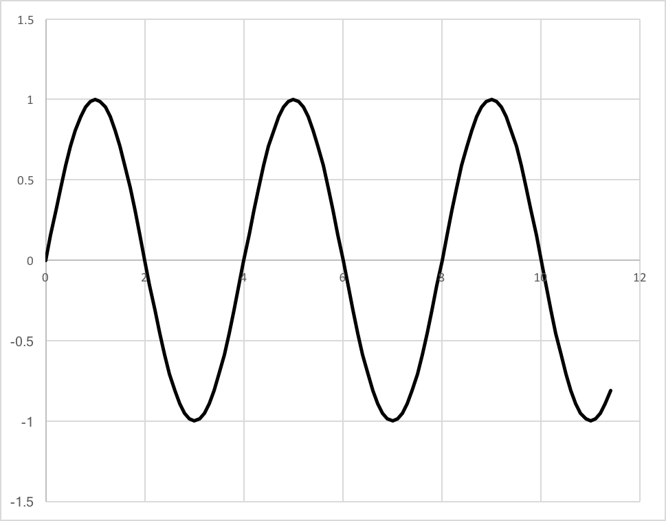
Now imagine that the physics you want to get to involves understanding the power spectrum as a function of frequency for the incoming wave, so you will want to execute a Fourier transform on the incoming signal. Normally, what you might do is to build electronics that uses an ADC to digitize the incoming signal at some time interval that is small compared to the period of the incoming wave. So if you took some data over a time period of several wavelengths, you would see a series voltage measurements at successive time intervals, and if you made a plot of the voltage at the given times you might see something like this:

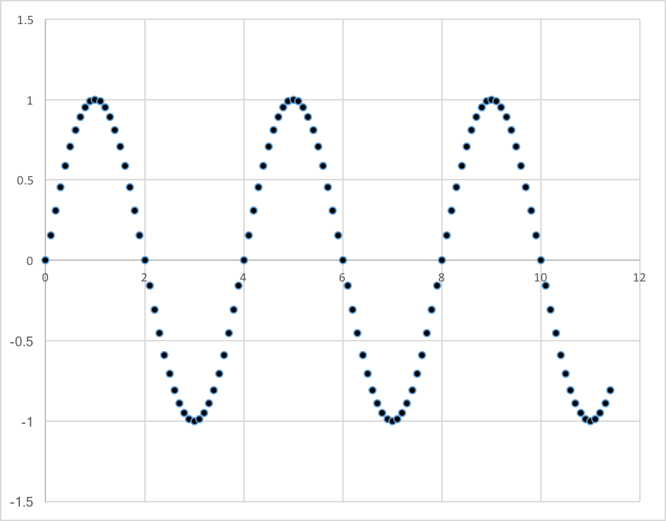
What you might want to do is use this data to measure the frequency of the incoming signal. So far this is pretty easy - if you applied a simple fourier transform to this data, you would get the right value. The only caveat is that the time between measurements is small compared to the period of the incoming signal. This is the Nyquist theorem: if δt is the time between measurements, and f is the frequency of the signal you want to sample (period T, then Nyquist requires that 1/δt ≥2f, or δt ≤ ½T.

In the real world, the incoming signals will be subject to two important effects: noise, and efficiency. By "noise", what is meant is that what is measured will be the sum (remember the principle of superposition) of a signal, plus stuff that is not only independent to the signal, but random in nature. By "efficiency", what is meant is that there is some probability different from 1 that given a signal, you actually see it. This probability can be near 0 (inefficient) or near 1 (completely efficient).

First, the noise. Imagine that the signal you are measuring is some waveform with sopme frequency $f$ and amplitude $A$ represented by $$S(t) = A\sin\omega t\nonumber$$ The noise can be distributed uniformly in some interval of amplitude, $\delta A$. If the interval $\delta A$ is small compared to the amplitude of the signal (A), say $\delta A = 0.1A$, then the combined signal would look like this:

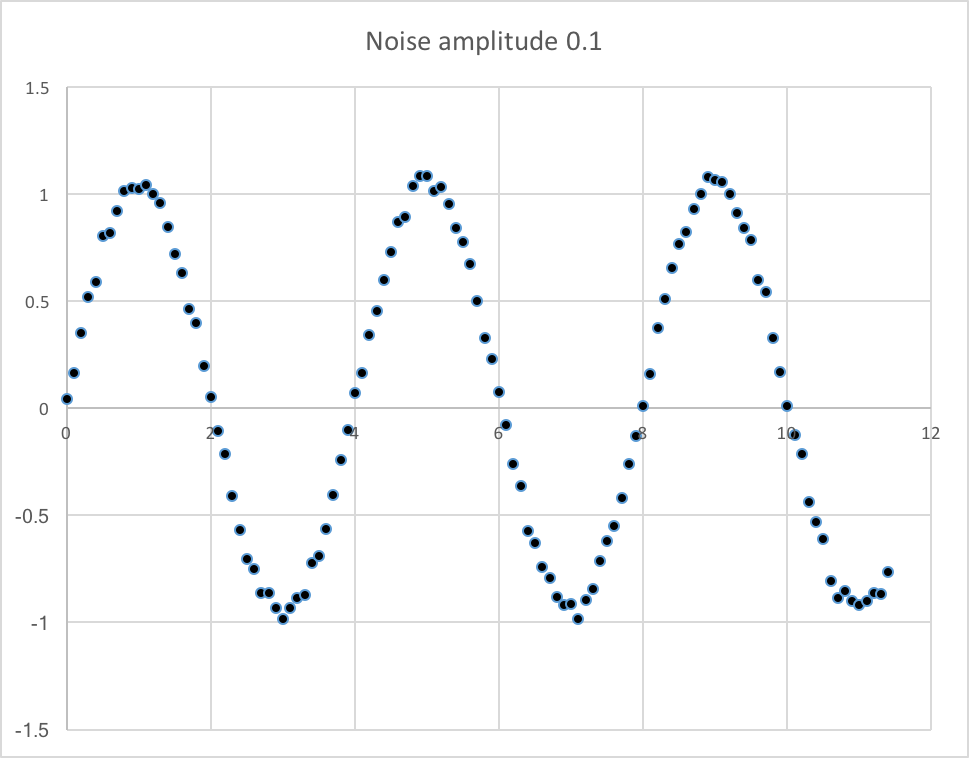
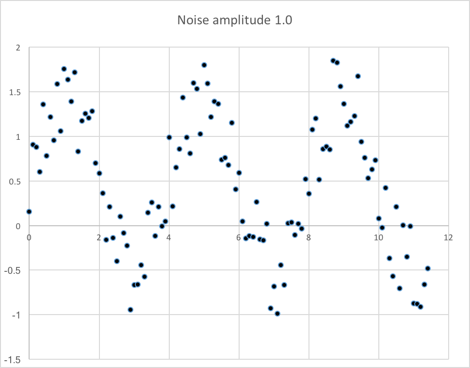
Pretty noisy data, however you can still clearly see the oscillation, and it's easy to estimate the period of oscillation. But you can cearly see that high levels of noise will wash out the signal, so let's try $\delta A = 5.0A$:

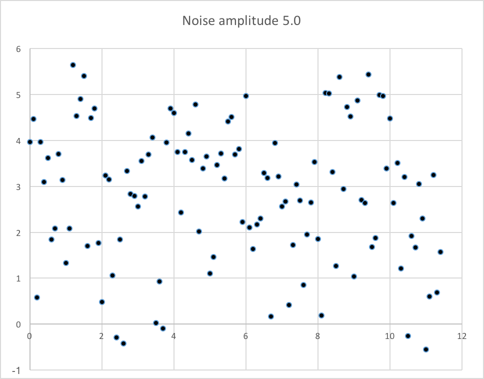
Not so good. You will need to do some kind of fourier analysis to see what frequencies can be fit into this.

Now let's consider efficiency. By efficiency, we mean that the signal you are trying to detect might, or might not, be present. For instance, imagine you have a telescope and you are pointing it at a very distant galaxy, and imagine the telescope has a very small area of view, so that it's looking only at that particular galaxy. That galaxy is so far away that any photon emitted would have to be exquisitely pointed at the earth in order to make it. Anything in between earth and the galaxy that deflects the photon by even the smallest amount will cause the photon to miss the telescope. So if the galaxy were to emit a continuous stream of photons, each one would have a finite probability of being detected, which means that the data you collect at some time interval might be data + noise, or it might be only noise, because the data has a finite detection efficiency.

In the simulation below, you can see an incoming sine wave after digitization. You can use the sliders to change the noise level (random noise, with amplitude relative to the wave amplitude) and the detection efficiency, and see how the incoming signal begins to look less like a periodic waveform and more like random noise.

The challenge is to dig the real signal out of the signal+noise. To illustrate this challenge, the following picture shows many periods of the incoming wave:

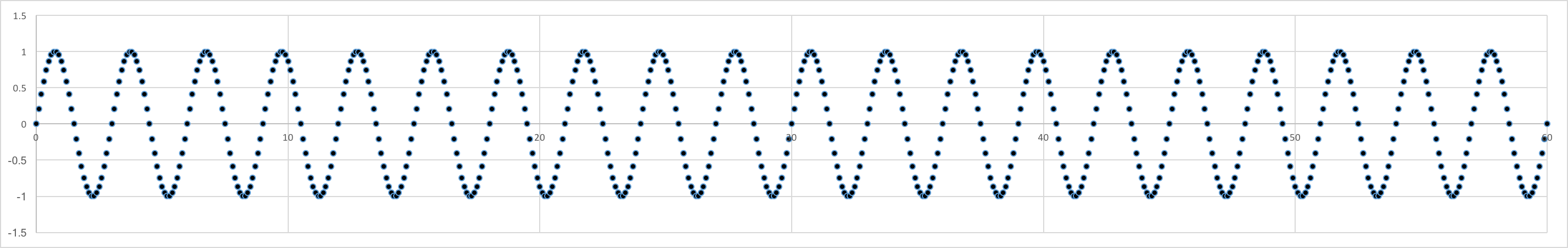
Image we have all those samples (each dot), with a sampling time $\delta t$, but we do not know the period or the phase of the incoming wave. So we capture $N_{int}$ samples in a row, and fourier analyze. Sounds fine, but if there's a great deal of noise and if the efficiency isn't so high, then we simply increase the number of points captured, and fourier analyze the result.

The problem with this is that you might need to capture quite a large amount of data, which means you will have to have a lot of resources (memory, FIFO, disk space, CPU) to fourier analyze the result. This becomes unpractical as the number of data points needed gets large, and that will happen if the noise is high and the efficiency is low.

One way to overcome the above problem would be to come up with some way to integrate the signal in real time as you collect data. Try the above simulation, setting the noise amplitude and efficiency and check the "Integrate?" checkbox, and hit generate many times. Even if you set the noise high and the efficiency low, eventually you will start to see a signal.

But integrating is not so straightforward, as you don't know the phase of the wave you are digitizing and adding to the previous waves. So adding successive $N_{int}$ number of points together will not necessarily happen coherently. In the above simulation, if you don't check "Random $\phi$?", then each digitized wave will have the same phase and that's why integrating works. If you check "Random $\phi$?", then integrating won't give you a signal no matter how many times you hit Generate.

The ideal solution would allow you to collect incoming digitized data and integrate in some way that's insensitive to the phase, and allows you to do so without having to take huge numbers of data and do fourier analysis on some kind of integrated sum. This can be done, and involves what is known mathematically as convolution.

To figure this out, let's start with 2 waves that have the same frequency but with a phase difference, $\phi$: $S_1(t) = A\sin(\omega t)$ and $S_1(t) = A\sin(\omega t + \phi)$. Then when we add them together, we get $$S_1 + S_2 = 2A\cos(\phi/2)\sin(\omega t)\nonumber$$ Now, let's suppose that the phase difference $\phi$ was just due to some time delay between the 2 waves, $\delta t$. That means that $\phi = \omega\delta t$, which means that the sum would be $2A\cos(\omega \delta t/2)\sin(\omega t)$. If we were to add up the 2 waves with a time delay that is equal to an integer times $\pi$, or equivalently $\delta t = nT$ where $n$ is an integer and $T$ is the period of the wave, the integral will be large and we would get a coherent sum. Since we can't know what time offset $\delta t$ to use, all we have to do is integrate with various values for the time offset, and the one where the integral is large will tell us the period of the incoming wave.

Voila, this is called a "convolution" of 2 functions, defined mathematically as: $$(f\circ g)(t) = \int_0^t f(t-\tau)g(\tau)d\tau\nonumber$$ However in our case, the 2 functions are the same, hence the "auto" in autocorrelation. We then have to build circuits that correlate an incoming signal with itself many times, each with a different delay.

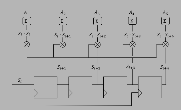
In the FPGA, the autocorrelator looks like the following figure. In this implementation, the incoming signal $S_i = S(t_i)$ is a single bit, and there are 5 states of correlation. The clock frequency for the shift register is $1/delta t$, and each time there's a new reading, you shift again, so that after $N$ readings, $S_i$ is shifted all of the way through. After each shift, the next data point $S_i$ is multiplied by the shifted value ($S_{i+1}, S_{i+2}$, etc) forming $S_i\cdot S_{i+1}$ and so on. Then we keep summing at each shift stage to produce $A_k, k=1,N$. This is the digital equivalent to the equation above for $(f\circ f)$.

The controls below allow you to simulate an incoming signal inside an FPGA autocorrelator. You can set the amplitude and period of each, and add noise and efficiency. You can think of the amplitude as being in arbitrary length units, and the period in seconds. The system will use a 10Hz clock, or a clock with a 0.1s period, producing a digital (discretized) signal every 0.1s. The conversion from analog produces a digital value, and you can change the number of bits used for the ADC, initially set to 1. You can change the number of bits to as large as 10, which means that the ADC will produce 1024 different values, which means each bit will mean 1/1024 of the total amplitude. The default is 1 bit might be surprising, as that means the FPGA would just be testing whether the signal was above or below some threshold, which does not give much resolution. But you will find that for many purposes, 1 bit is enough to see the relevant spectrum if you integrate long enough.

You can also turn on noise with an amplitude (same units) and you can employ an efficiency for the incoming signal (not the noise, of course). Hit the Start button to start, and you can change things dynamically but it is usually better to hit Reset (equivalent to Stop with a reset of the spectrum sums) between changing parameters. The simulation is pretty good at showing the power of autocorrelation!

As you can see, the autocorrelation takes an incoming signal and produces a signal that over time eliminates the noise and leaves only what's repeating (oscillating). But to get the frequency components of the incoming signal, which is what you want to know, you have to do a fourier analysis on the autocorrelated signal. The last button on the right is labeled "Fourier". When you hit this button, it will execute a discrete fourier analysis (see A Thinking Person's Guide to Fourier Analysis and Fourier analysis on Wikipedia) and display the coefficients for the cosine (even) and sine (odd) basis functions. You can see a few things clearly here:

• You should see a peak at the incoming frequency $f=1/T$
• Since the data is real, we have the constraint that the maximum frequency we can measure is the Nyquist frequency given by $f_c = 1/2\delta t$, so we only plot the first $N/2$ frequencies.
• You can run the simulation with 1, 2, 3, etc bits, and observe the coefficients $a_n$ for the even functions and $b_n$ for the odd functions. You can see that for a 1-bit ADC, you will see a few more frequencies than just the main harmonic. This is due to the quantization error. When you get up to 2 or 3 bits, these extra frequencies will be diminished a great deal.

FPGA Autocorrelator

Here we will build an autocorrelator circuit with a 1-bit ADC. We can do this easily by digitizing the incoming analog audio signal using the Electret, and compare to a threshold. If the signal is above, then the output is 1, and if it's below, the output is 0. Our Electret has a DC offset, so we will first measure the offset by injecting a sine wave tone into the Electret microphone and reading out data from the FIFO and taking an average. In a more controlled experiment, we could build an audio amplifier that ensures the average signal will be at half range, but for now, we will have to just measure the range of the signal do calculate the average. Then download the threshold to a new register, which we can call the threshold register and place this inside the controller.v module like in the following code (we can put it right after the status register is declared):

    //
    //  threshold register for 1-bit ADC for the correlator
    //
    reg [11:0] threshold = 12'h9eb;
    wire digitized = adc_data > threshold ? 1 : 0;

Note that the wire digitized will be what we send into the autocorrelator (see below).

Remember that the XADC will digitize every 22.676μs (1/44.1kHz), with the resulting ADC value latched into the signal r_adc_data which is sent into the controller.v module and renamed adc_data. So we can built our autocorrelator into controller.v and not have to change top.v or any other module.

So far the only signals the RPi sends to the FPGA is the control register and the blast register, so we will need to add threshold. The control register comes in at address 0x1, the blast register at 0x3, so we will use 0x5 for the threshold register. We will also want to read it back, and we will put that command address at the next empty one, which will be 0x10. So the top of controller.v should be changed (only the comments actually, the line that reads "0000 0101" and "0001 0000") to this:

//////////////////////////////////////////////////////////////////////////////////
//
//  this module assumes that in the level above, there's a FIFO that buffers all
//  UART receive transmissions.
//
//  the rx_data contains the relevant data to decode:
//
//  7654 3210
//              LSB=1 means the RPi is sending info that will come on the next transmission
//              All transactions are 8 bits 
//  0000 0001   RPi is sending control register (on/off...etc)
//  0000 0011   "    "   "     blast register
//  0000 0101   "    "   "     threshold register
//
//              LSB=0 means RPi wants FPGA to send stuff back
//  0000 0010   send back 16 bit ADC value from XADC block directly
//  0000 0100   send back 16 bit test value from slide switches
//  0000 0110   send back 16 bit firmware version
//  0000 1000   send back 8 bit control register (upper 8 bits are all zero)
//  0000 1010   send back 8 bit status register (ditto)
//  0000 1100   semd back 16 bit blast register
//  0000 1110   send back the ADC data fifo counts
//  0001 0000   send back the threshold register value
//  1000 0000   blast back 65536 data points from ADC fifo or until empty
//
module controller(
    input clock25,              // 25MHz input clock to match uart_rx and uart_tx clock and adc fifo read
    input fifo_clock,           // fifo input clock, which should be 44.1kHz
    input reset,                // reset (BTNR)
    output global_start,        // drive one of the LEDs with this line
    //
    //  rx fifo stuff
    //
    input rx_fifo_empty,        // fifo empty
    input [7:0] rx_fifo_data,   // 8 bits of fifo data
    output rx_fifo_rd_en,       // fifo read enable
    //
    //  uart_tx stuff
    //
    output [15:0] tx_transmit_out,      //  2 bytes to send out
    output tx_transmit,                 //  signal to send them
    input tx_done,                      //  asserted twice per transfer
    //
    //  data inputs
    //
    input [15:0] version,           //  set at the top of top.v
    input [15:0] test,              //  slide switches
    input [15:0] adc_data,          //  latched into r_adc_data
    //
    //  ADC fifo stuff
    //
    input adc_fifo_empty,                   //  fifo empty
    input adc_fifo_full,                    //  fifo full
    output reg adc_fifo_rd,                 //  read enable
    output adc_fifo_wr,                     //  write enable
    input [15:0] adc_fifo_data_count,       //  number left to read
    input [15:0] adc_fifo_data,             //  all 16 bits of data
    //
    //  debug
    //
    output [49:0] debug
    );

We will make the threshold register 12 bits, since that is what we will be comparing to the upper 12 bits of the adc_data value. The top 12 bits of the incoming (to controller.v) bus adc_data will be compared to the threshold to produce a 1-bit "adc" that will be sumed in our correlator. The code for the threshold register and "digitized" sum will be:

    //
    //  threshold register for 1-bit ADC for the correlator
    //
    reg [11:0] threshold = 12'h9eb;
    wire digitized = adc_data[15:4] > threshold ? 1 : 0;

Let's put this code right after the control register, inside controller.v.

We will want to have this register programmable via the uart interface between the RPi and the FPGA. To accommodate this register, the IN state machine code will have to be changed by making incoming_what be 2 bits, and in the case statement adding latching in_data into threshold:

    //
    //  here is the "incoming" FSM that responds to the RPi sending data to the FPGA
    //
    localparam [3:0] IN_WAIT=0, IN_WAIT_NOT_EMPTY1=1, IN_READ1_EN1=2, IN_READ1_EN0=3, IN_READ1_LATCH=4,
        IN_WAIT_NOT_EMPTY2=5, IN_READ2_EN1=6, IN_READ2_EN0=7, IN_READ2_LATCH=8, IN_DONE=9;
    reg [3:0] in_state;
    reg in_read_fifo;
    reg in_done;
    reg [15:0] in_data;
    reg [1:0] incoming_what;
    always @ (posedge clock25)
        if (reset) begin
            in_state <= IN_WAIT;
            in_read_fifo <= 0;
            in_data <= 0;
            in_done <= 0;
            incoming_what <= 0;
        end
        else case (in_state) 
            IN_WAIT: begin
                in_read_fifo <= 0;
                in_data <= 0;
                in_done <= 0;
                in_state <= do_incoming ? IN_WAIT_NOT_EMPTY1 : IN_WAIT;
                incoming_what <= rx_instructions[2:1];    // what incoming is coming in
                end
            IN_WAIT_NOT_EMPTY1: begin
                in_state <= incoming ? IN_READ1_EN1 : IN_WAIT_NOT_EMPTY1;
            end
            IN_READ1_EN1: begin
                in_read_fifo <= 1;
                in_state <= IN_READ1_EN0;
            end
            IN_READ1_EN0: begin
                in_read_fifo <= 0;
                in_state <= IN_READ1_LATCH;
            end
            IN_READ1_LATCH: begin
                in_data[7:0] <= rx_fifo_data;
                in_state <= IN_WAIT_NOT_EMPTY2;
            end
            IN_WAIT_NOT_EMPTY2: begin
                in_state <= incoming ? IN_READ2_EN1 : IN_WAIT_NOT_EMPTY2;
            end
            IN_READ2_EN1: begin
                in_read_fifo <= 1;
                in_state <= IN_READ2_EN0;
            end
            IN_READ2_EN0: begin
                in_read_fifo <= 0;
                in_state <= IN_READ2_LATCH;
            end
            IN_READ2_LATCH: begin
                in_data[15:8] <= rx_fifo_data;
                in_state <= IN_DONE;
            end
            IN_DONE: begin
                //
                //  here is where we latch according to what the RPi wants to send
                //
                in_done <= 1;
                case (incoming_what)
                    2'b00: control <= in_data;
                    2'b01: blast <= in_data;
                    2'b10: threshold <= in_data[11:0];
                    default: control <= in_data;
                endcase
                in_state <= do_incoming ? IN_DONE : IN_WAIT;
            end
        endcase
    assign incoming_done = in_done;

Similarly, we will also want to read the threshold register into the RPi. So the OUT state machine code will also have to be modified so that outgoing_what is increased to 3 bits and threshold is added to the list of registers that can be sent out:

    //
    //  now make the state machine to handle sending 16 bit words to the RPi
    //    
    localparam [2:0] OUT_WAIT=0, OUT_LATCH=1, OUT_TRANSMIT=2, 
        OUT_TRANSMIT_WAIT1=3, OUT_TRANSMIT_WAIT2=4, OUT_DONE=5;
    reg [2:0] out_state;
    reg [15:0] tx_out;
    reg transmit_out;
    reg out_done;
    reg [3:0] outgoing_what;
    always @ (posedge clock25)
        if (reset) begin
            out_state <= OUT_WAIT;
            transmit_out <= 0;
            out_done <= 0;
            tx_out <= 0;
            outgoing_what <= 0;
        end
        else case (out_state)
            OUT_WAIT: begin
                transmit_out <= 0;
                tx_out <= 0;
                out_done <= 0;
                out_state <= do_outgoing ? OUT_LATCH : OUT_WAIT;
                outgoing_what <= rx_instructions[4:1];    // what is going out (only need 4 bits for now)
            end
            OUT_LATCH: begin
                case (outgoing_what)
                    4'b0001: tx_out <= adc_data;
                    4'b0010: tx_out <= test;
                    4'b0011: tx_out <= version;
                    4'b0100: tx_out <= control;
                    4'b0101: tx_out <= status;
                    4'b0110: tx_out <= blast;
                    4'b0111: tx_out <= adc_fifo_data_count;
                    4'b1000: tx_out <= {4'b0,threshold};
                    default: tx_out <= 16'hDEAD;    // error!
                endcase
                out_state <= OUT_TRANSMIT;
            end
            OUT_TRANSMIT: begin
                transmit_out <= 1;
                out_state <= OUT_TRANSMIT_WAIT1;
            end
            OUT_TRANSMIT_WAIT1: begin
                transmit_out <= 0;
                out_state <= tx_done ? OUT_TRANSMIT_WAIT2 : OUT_TRANSMIT_WAIT1 ;
            end
            OUT_TRANSMIT_WAIT2: begin
                out_state <= tx_done ? OUT_DONE : OUT_TRANSMIT_WAIT2;                
            end
            OUT_DONE: begin
                out_done <= 1;
                out_state <= do_outgoing ? OUT_DONE : OUT_WAIT;                
            end
        endcase
        assign outgoing_done = out_done;

Depth

The more stages you have, the lower the frequency you can detect. So if we decide that we won't want to detect anything lower than say 100Hz, or signals that are more than 0.01s apart, then the depth will be given by the minimum frequency (here 40Hz) divided into the time between samples, or 1/44.1kHz. That gives us 44.1kHz/100Hz = 441 stages. That may seem like a lot of flip-flips and memory, but then the Artix 7 has plenty of resources. Also note that the autocorrelation happens at the same rate as the 44.1kHz digitization clock, with a period of 22.67μs, and inside an FPGA, that's an eternity compared to the 10ns system clock.

Width

At each state, we want to multiply the value of the bit at that stage in the shift register with the incoming bit, and add to a sum. The sum will accumulate accordingly. So we have to consider how many bits in each sum, aka "width". Now each value added to the sum is either a 0 or a 1 for a 1-bit autocorrelator, so if our width is, e.g., 16 bits, and each bit is added at 44.1kHz, then if each bit added is a 1, the number of seconds it will take to saturate the sum so that it has a value 0xFFFF will be $2^{16}\times (1/44100Hz) = 1.486$ sec. That doesn't seem like enough time. But if we multiply this by 3600, we will have 1.486 hours, which does seems like enough time. 3600 is approximately $2^12$ so if we have 28 bit sums, then we can integrate for around 1.7 hours, which should be plenty. But let's just make the sums 32 bits, as that will make it easier to read each half (remembering that the FPGA and RPi always send or receive 8 bits at a time). That means we can integrate for at least $2^32\times (1/44100Hz) = 27 hours, which should be way more than enough.

Total bits

The total number of memory bits needed will be dominated by the sums, which will be the width of each sum times the number of sums, so for the above guess, we will need $441\times 32 = 14112$ bits. The Artix 7 has 215k logic cells and 13Mb BRAM, and the 215k gives us plenty of room to put all the memory into SRAM and not have to take up BRAM, which would be more difficult to code up.

The verilog code for making a shift register is pretty straight forward. Let's start with a shift register with 4 stage, and let adc be the 1-bit of incoming data.

    module correlator (
        input clock,
        input adc
    );
    reg [3:0] shift;
    always @ (posedge clock) begin
        shift[0] <= adc;
        shift[1] <= shift[0];
        shift[2] <= shift[1];
        shift[3] <= shift[2];
    end
    endmodule

    module correlator (
        input clock,
        input adc
    );
    integer i;
    reg [3:0] shift;
    always @ (posedge clock) begin
        shift[0] <= adc;
        for (i=0; i<3; i++) begin
            shift[i+1] <= shift[i];
        end
    endmodule

Note the first line, integer i;. That is a non-executable instruction. It just tells the compiler to set aside an integer to be used for loops. And inside the always block we see the syntax for (i=0; i<4; i++), just like in c++ or javascript. Here you see how the integer i is used as a pointer inside the for loop. Also note that the register shift is declared as 3:0, or 4 bits. Inside the for loop, we want "i<3" so that the last value is 2, and the next line would give us shift[3] <= shift[2], which is what we want.

Our code for the 441 stages is pretty simple, and starts with this:

    module correlator (
        input clock,
        input adc
    );
    integer i;
    reg [881:0] shift;
    always @ (posedge clock) begin
        shift[0] <= adc;
        for (i=0; i<881; i++) begin
            shift[i+1] <= shift[i];
        end
    endmodule

The above code is just a shift register, so now let's turn this into a correlator by adding sums. Here we make use of the verilog way of defining arrays of registers that have a width greater than 1:

    reg [7:0] sums[0:9];

The signal sums is defined as an array of 8 bit registers (the [7:0]), and that there are 10 of them, going from 0 to 9 (sums[0:9]). Note that the register length declaration has the MSB:LSB pattern, but the indexing of the sums is just 0 to 9 in that order. What we want to do is to sum over the product of the value after each shift times the incoming data adc, which here is 1 bit. The product of 2 1-bit numbers is either 0 or 1, and its 1 only when both are 1, which is the same as an AND gate.

    module correlator (
        input clock,
        input adc
    );
    integer i;
    reg [881:0] shift;
    reg [7:0] sums[0:9];
    always @ (posedge clock) begin
        shift[0] <= adc;
        for (i=0; i<881; i++) begin
            shift[i+1] <= shift[i];
            sums[i] = sums[i] + (shift[0] & shift[i]);
        end
    endmodule

Let's add an enable input as well, so that we can turn the correlation on and off, and a reset to set everything to a known value.

module correlator (
    input clock,
    input reset,
    input enable,
    input adc
    );
    integer i;
    reg [7:0] sums[0:9];
    reg [9:0] shift;
    always @ (posedge clock)
        if (reset) begin
            shift <= 0;
            for (i=0; i<10; i=i+1) begin
                sums[i] <= 0;
            end
        end
        else begin
            if (enable) begin
                shift[0] <= adc;
                for (i=0; i<10; i=i+1) begin
                    shift[i+1] <= shift[i];
                    sums[i] = sums[i] + (shift[0] & shift[i]);
               end
            end
        end
endmodule

Now let's change sum width and number of stages to become parameters, so that we can use the code for other purposes. We do this by making use of the verilog `define statement, which defines a parameter:

`define SUM_WIDTH 8
`define STAGES 32
module correlator (
    input clock,
    input reset,
    input enable,
    input adc
    );
    
    integer i;
    reg [`SUM_WIDTH-1:0] sums[0:`STAGES-1];
    reg [`STAGES-1:0] shift;
    always @ (posedge clock)
        if (reset) begin
            shift <= 0;
            for (i=0; i<`STAGES; i=i+1) begin
                sums[i] <= 0;
            end
        end
        else begin
            if (enable) begin
                shift[0] <= adc;
                for (i=0; i<`STAGES; i=i+1) begin
                    shift[i+1] <= shift[i];
                    sums[i] = sums[i] + (shift[0] & shift[i]);
               end
            end
        end
endmodule

So at the top we use `define SUM_WIDTH 8 to be the width of the sums, and `define STAGES 32 to have 32 stages of shifting, which means 32 sums. Then when declaring the sum registers, we use `SUM_WIDTH-1 (which is 7) to declare 8-bit registers, and `STAGES to make 32 of then. So the statement:

    reg [7:0] sums[0:31];
    reg [31:0] shift;

is equivalent to

    `define SUM_WIDTH 8
    `define STAGES 32
    reg [`SUM_WIDTH-1:0] sums[0:`STAGES-1];
    reg [`STAGES-1:0] shift;

One last twist: we often need parameters in more than 1 module. The easiest thing to do is to define a new verilog module, let's call it include.v, and in this module you put the 2 `define statements. Then, in the verilog module that needs them, you simply add them to the top using the verilog `include statement like this:

    `include "include.v"
    module (...
    );
    ...
    endmodule

For our autocorrelator project, we will set SUM_WIDTH to 32 bits and STAGES to 441, so the include.v file will look like this:

`define SUM_WIDTH 32
`define STAGES 441

and we can include it in both autocorrelator.v and in controller.v (see below).

We can simulate the above code using the Vivado simulation, and writing a testbench, which will look like this:

`timescale 1ns / 1ps
module top_tb;
    reg clock, reset, adc, enable;
    
    correlator MYCORR (
        .clock(clock),
        .reset(reset),
        .enable(enable),
        .adc(adc)
        );

    parameter PERIOD = 10.0;
    always begin
        clock = 1'b0;
        #(PERIOD/2) clock = 1'b1;
        #(PERIOD/2);
    end 
    
    integer i;
    initial begin
        reset = 0;
        adc = 0;
        enable = 0;
        #100 reset = 1;
        #10 reset = 0;
        #100;
        enable = 1;
        for (i=0; i<100; i=i+1) begin
            adc = 0;
            #10 adc = 1;
            #10 adc = 1;
            #10 adc = 0;
            #10;
        end

        #10 enable = 0;        
    end

endmodule

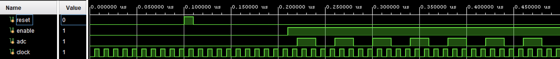
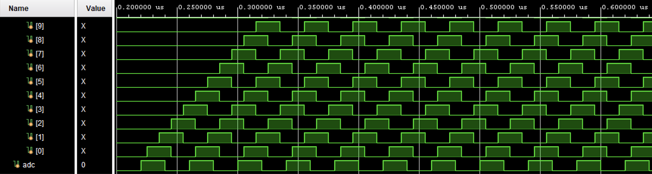
The period is set to 10.0, and since the `timescale is 1ns, that's 10ns, or 100MHz clock. In the "initial" block, we set everything to a definite value, then wait 100ns and hit the reset for 1 clock cycle, then wait another 100ns and inside the for loop, we drive adc to 0, then 1, then 1, then 0, and do that 100 times. So this inputs data that is periodic, with period 4x10ns = 40ns. In the figure below, you can see the reset go high for 1 clock period at 100ns, then a 100ns pause, then enable goes high, and adc goes high for 2 clock ticks, low for 2, and so on.

The next figure shows the shift register, and the data being shifted (shift[0] is on the bottom, and going up the page you see more shift registers, here we only show the first 10).

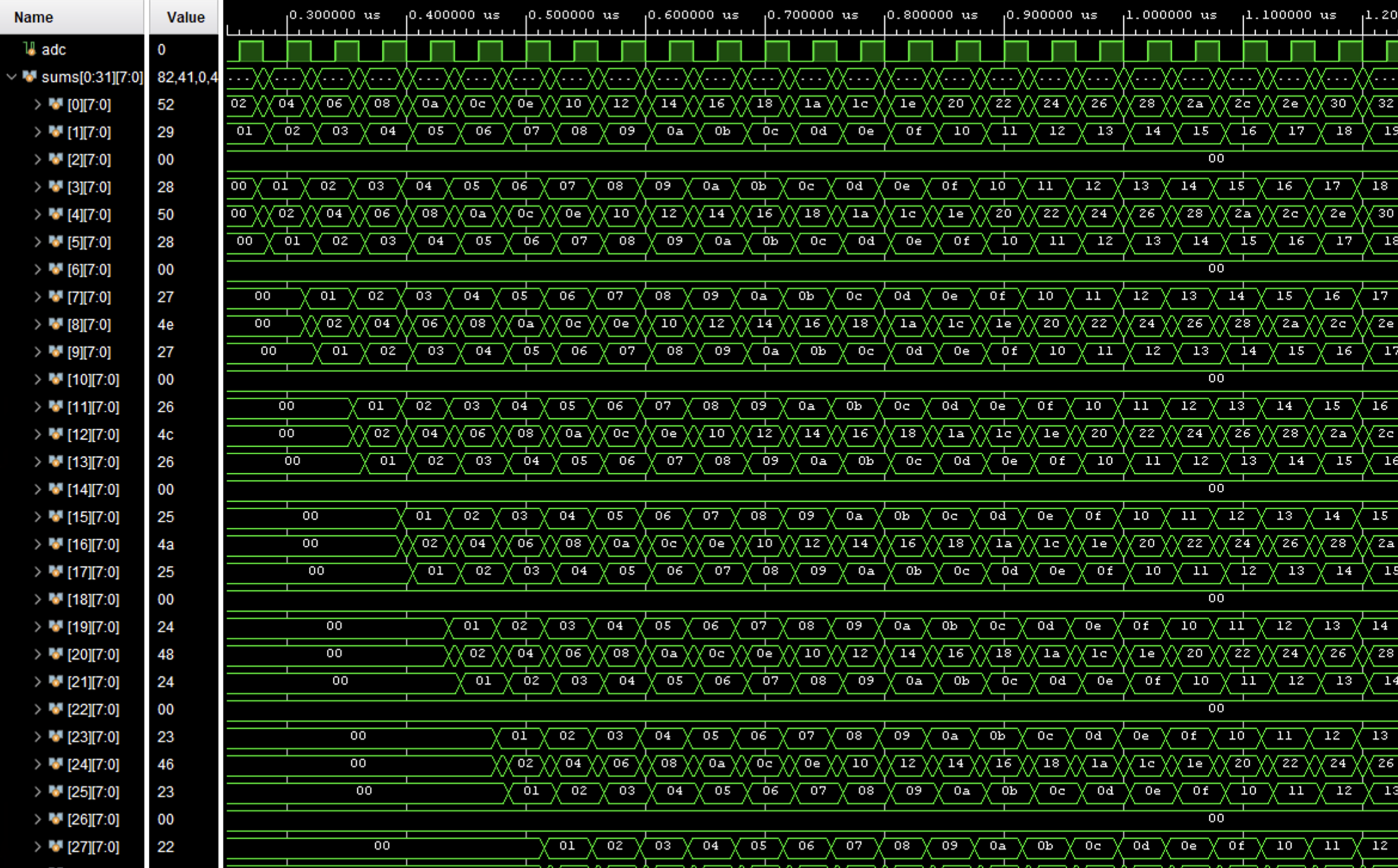
Finally, the next figure shows the sums, where the 1st sum is at the top. You can see that the sums have a repetition of 4.

That tells you that the period of the incoming wave is 4 ticks, or 40ns, which is what we set in our testbench.

We are now ready to add the autocorrelator to our audio project, where we have started with the project made for the Increasing Bandwidth lab and added a threshold register. The first thing we should do is to figure out how we are going to be able to read out all of the autocorrelator sums. Since we are talking about something like 441 sums, each of which is something like 32 bits wide, we have to come up with some scheme for the RPi to tell the FPGA which sum, and which part of which sum. So let's invent a register inside FPGA that will tell it which sum to send, and call this register sumid. It will have to be at least 9 bits long to be able to identify which of the 441 registers, so let's make it 16 bits long since the RPi sends 8 bits at a time. So we add this line to the comments at the top of controller.v:

//  0000 0111   "    "   "     sumid register

and this code below where we inserted the 12 bit threshold register:

    //
    //  sumid register, which tells the autocorrelator which sum to send to the RPi
    //
    reg [15:0] sumid = 0;

and this to the case statement inside the IN state machine to capture the register:

    2'b11: sumid <= in_data;

There's probably no need to read the sumid register back so we won't bother changing the OUT state machine like we did for the threshold register.

All we have to do is to pass as an input the sumid value to autocorrelator.v module, and output the sum that sumid points to. So our autocorrelator.v will look like this:

`timescale 1ns / 1ps
`include "include.v"

module autocorrelator (
    input clock,
    input reset,
    input enable,
    input adc,
    input [9:0] sum_id,
    output [`SUM_WIDTH-1:0] sum_out
    );
    
    integer i;
    reg [`SUM_WIDTH-1:0] sums[0:`STAGES-1];
    assign sum_out = sums[sum_id];
    reg [`STAGES-1:0] shift;
    always @ (posedge clock)
        if (reset) begin
            shift <= 0;
            for (i=0; i<`STAGES; i=i+1) begin
                sums[i] <= 0;
            end
        end
        else begin
            if (enable) begin
                shift[0] <= adc;
                for (i=0; i<`STAGES; i=i+1) begin
                    shift[i+1] <= shift[i];
                    sums[i] = sums[i] + (shift[0] & shift[i]);
               end
            end
        end
endmodule

Before we instantiate the correlator module inside controller.v, let's add another 2 bits to the control register to enable the correlator sums, and to allow the RPi to reset the sums inside correlator without you having to push the reset button on the FPGA BASYS3 board. Note that the reset inside autocorrelator.v is synchronous with the clock because the statement

always @ (posedge clock) ...

controls what happens to the reset condition. We could change it to an asychronous reset by changing the code to be:

always @ (posedge clock or posedge reset) ...

Anyway we can do either, but if you do a synchronous reset, you have to make sure that the reset signal is at least as wide as 1 clock tick or the code could miss it, since it only checks at the posedge.

Either way, we will have to have the RPi set a bit in the controller that is immediately cleared. We can clear this bit in software or firmware, but software might be easier. (Don't forget!!!)

In the controller.v module, define a new wire called reset_corr for resetting the autorcorrelator:

    //
    //  here is the control register, however the RPi serial input buffer is only 4096
    //  bytes deep.  So we only want to be blasting 2048-1 (starrting from 0) = 0x7FF 
    //  16-bit words at a time
    //
    reg [15:0] control = 0;
    assign global_start = control[0];
    assign test_mode = control[1];
    assign correlator_enable = control[2];
    assign reset_corr = control[3];

We are ready to instantiate this in controller.v using the following code (I placed it right after defining sumid):

    //
    //  instantiate the autocorrelator module here
    //
    wire [`SUM_WIDTH-1:0] sumout;
    autocorrelator CORR (
        .clock(fifo_clock),
        .reset(reset_corr),
        .enable(correlator_enable),
        .adc(digitized),
        .sum_id(sumid),
        .sum_out(sumout)
    );

Next, we have to add the code to controller.v to send the sum that sumid points to back to the RPi, so that all the RPi has to do is just loop through reading each sum. This won't be as fast as the "blasting" of data from the FIFO. In a previous lab, Digital Oscilloscope, we found that the time it takes for the RPi to send data to the FPGA asking for something, plus the time to get 2 bytes back, is around 45μs. Here the RPi will have to get 4 bytes per sum, so it will be around 90μs per request, times 441 sums which will take about 80ms, which is pretty quick even though it's a lot of data.

So we now need to add sending the sumout value back to the RPi, which means adding functionality to the OUT state machine. We will need 2 commands here, one for the lower 16 bits and one for the upper, so let's add the following to the comments section at the top of controller.v that says what the commands are:

//  0001 0010   send back lower 16 bits of sumout
//  0001 0100   send back upper 16 bits of sumout

and the following to the OUT state machine case statement:

    4'b1001: tx_out <= sumout[15:0];
    4'b1010: tx_out <= sumout[`SUM_WIDTH-1:16];

Note that we are using 32 bit sums inside autocorrelator,v, which is way overkill but convenient since we have to send the sums back to the RPi using the 8-bit serial path.

An alternative way to code up an autocorrelator would be to use block ram, to allow many more stages. The basic idea is that you can write to block ram at 100MHz, whereas the data is coming in at 44100Hz. So that means there are $100\times 10^6/44.1\times 10^3=2267$ system clock ticks between each new data. The shifting only takes a single clock tick, but block ram is such that you have to specify and address, then write. If the depth of the block ram is less than 2267, all you would have to do is loop over the addresses and write a new sum to each bram address. It won't be an easy thing to code, but it's doable. For now, let's do the easy thing and stick with using DRAM inside the FPGA as outlined above.

The 3 most important verilog sources are available:

• top.v
• controller.v
• autocorrelator.v

Python code

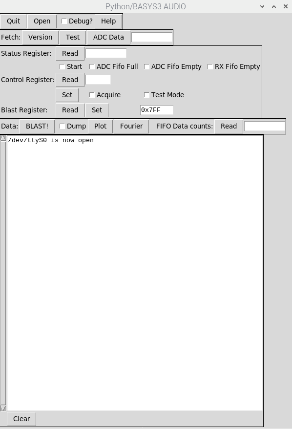
The python code for controlling the audio project is called audio.py and can be found here. When you run it on the RPi, you will see the following gui:

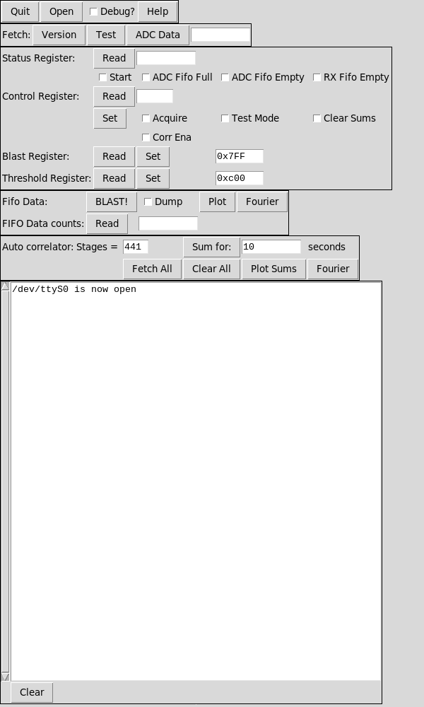
Once you have a signal into the XADC inputs (see Using the FPGA ADC), the first thing you have to do is to measure the average value of that signal so that you can set the threshold register. To do this, hit the "BLAST!" button and the code will tell the FPGA to fill the FIFO, then read out all values and report the average value as a voltage, integer, and hex number. (You can see the signal by hitting the "Plot" button to the right of "BLAST!", and look at the Fourier spectrum by hitting the "Fourier" button to the right of that). Then set the hex value of the "Threshold Register" in the text window to the right, and hit the "Set" button. It's a good idea to read it back to make sure it got it.

Once you have the threshold set, all you have to do is set the number of seconds you want to wait to fill the sums, and hit the "Sum for:" button. It will report "done!" when it's done. You can also control things by hand by checking "Corr Ena" under the "Control Register:", and hitting the "Set" button. Then hit the "Read" to make sure the right bit is set. Then wait however long you want, clear the "Corr Ena" button and hit "Set" again, and the sums will stay static.

To read the data from the FPGA, hit the "Fetch All" button to read all of the sums into an internal array (you can check the "Debug?" button on the top and it will show you all values as they are read in). When that's done, you can hit "Plot Sums" and then "Fourier" to analyze the spectrum.

I tested this using a 1kHz square wave that has a 1V peak-to-peak, and injected into the XADC inputs. When I hit "BLAST!", it takes around 5.7 seconds to fill all 65535 values into the FIFO, and reports that the average ADC value is 0x800 which corresponds to half scale (remember, the XADC is a 12 bit ADC, so full scale is 1 volts and that should be 0xFFF, so half scale is 0x7FFF which is pretty much the same as 0x800).

Hit the "Plot" button to the right of "BLAST!" and it will show you this plot of the FIFO ADC values it read back:

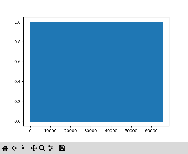
This is what you would expect from a 1kHz square wave - there are just too many wavelengths! So use the zoom feature and blow it up and you should see this:

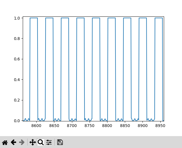
The input signal might be slightly greater than the maximum input for the XADC, but that's ok, it's a square wave after all. In the plot, the horizontal axis is the n'th data word in the FIFO, and the period looks to be around 44, which it should be since we have a 1kHz signal digitized at 44.1kHz, which means 44.1 pieces of data per period.

We can then hit the "Fourier" button to the right of "BLAST!" and look at the spectrum:

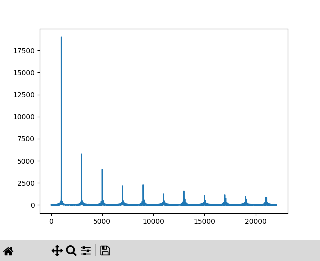
The analytical Fourier series of a square wave $f(t)$ with period $T$ (see A Thinking Person's Guide to Fourier Analysis for more) should be $$g(\omega) = \frac{4}{\pi}\sum_{n=odd}\frac{1}{n}\sin(n\omega t)\nonumber$$

The above plot looks pretty good for the first 4 components, then tends to flatten off, probably due to things like the input signal not being a perfect square, XADC digitization error, noise, etc.

Now let's run the autorcorrelator and compare. First set the threshold register text field to 0x800 and hit "Set" and "Read" to be sure it's set properly. Then hit "Sum for:" (10 seconds is enough, but feel free to use whatever value you want). After the 10 seconds is up, you can hit "Fetch All" to read all the values in (if you check the "Debug?" box at the top, it will show you the values it read in).

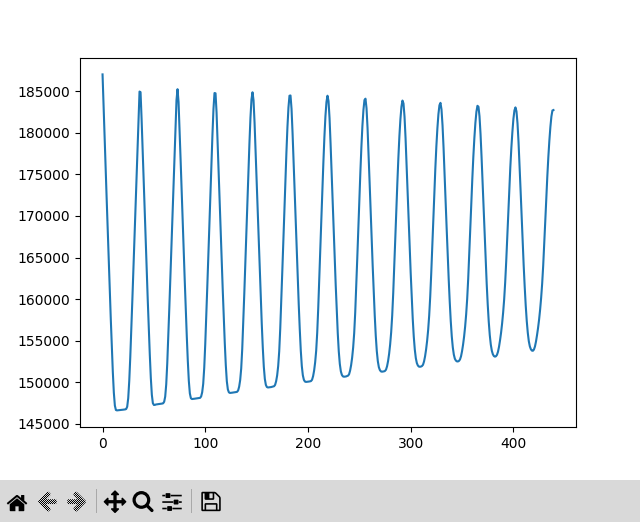
Hit the "Plot Sums" button underneath "Sum for:", and you should see the following plot:

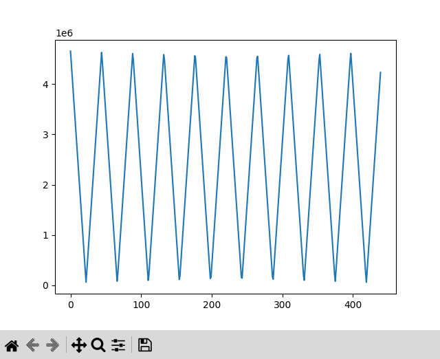
This is exactly the shape you would expect from an incoming square wave with no noise and no efficiency (see the above simulation).

To see the fourier analysis of the above sums, hit the "Fourier" button to the right of "Plot Sums". You should see something like this:

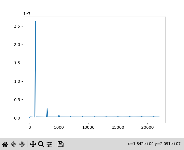
The large first peak is exactly at 1kHz, with some smaller harmonics due mostly to digitization (my guess). Full disclosure: when reading all of the raw sums, I am finding that the very last sum is identically 0, so in the code for audio.py, this element is removed, although it's not necessary for anything but esthetics, and when I have the time I will eventually debug it.

Another test you can do is to take data with the Electret connected to the XADC input, and whistle. I did this trying to keep a steady tone, which I measured to be around 1200Hz. I took 3 sec of sums. Here are the raw sums and fourier spectrum:

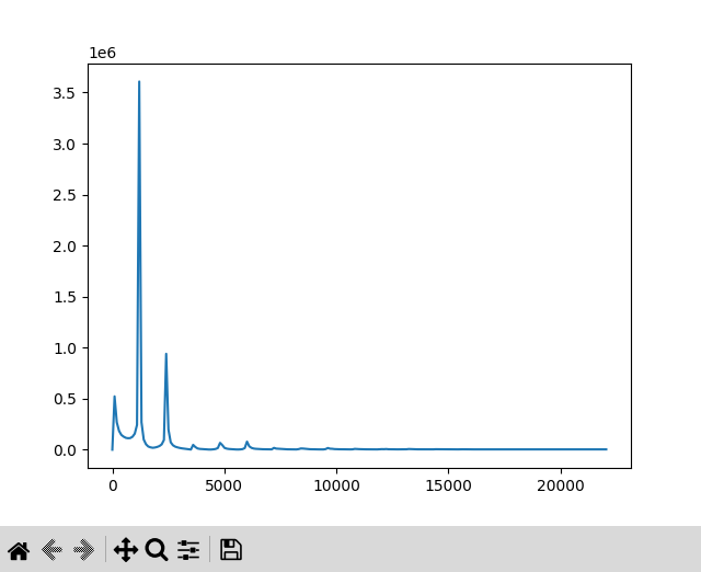
The large peak in the fourier spectrum is in the right place.