If is often the case that we want to write computer programs to simulate various physics processes. For example, starting simple, let's say we want to simulate a 2-dimensional ball moving at constant velocity across a rectangular area, and bounce off the walls, as in the figure below. The position of the ball has coordinates $(x,y)$, and the ball moves with velocity $\vec v$ in 2 dimensions, so we resolve the velocity into a velocity along the horizontal (x) direction, $\vec v_x$, and a velocity along the vertical (y) direction, $\vec v_y$. You can see clearly what happens when the ball hits the wall: the velocity perpendicular to the wall is reversed, and the velocity parallel to the wall is unchanged.
To simulate this, let's just focus on one dimension $x$ with velocity $v$ and ignore the subscript. We first use the definition of velocity: $$v = \frac{dx}{dt}\nonumber$$ To calculate the displacement along $x$ from position $x_1$ at time $t_1$ to position $x_2$ at time $t_2$, all we have to do is integrate the velocity: $$\int_{x_1}^{x_2} dx = \int_{t_1}^{t_2} v\cdot dt\nonumber$$ The left side of this equation is easy: $$\int_{x_1}^{x_2} dx = x_2 - x_1\nonumber$$ This gives us the equation: $$x_2 = x_1 + \int_{t_1}^{t_2} v\cdot dt\label{emaster}$$ Equation $\ref{emaster}$ tells us how to "swim" the position from position $x_1$ to position $x_2$. Voila, now you see why the subject of simulating physical systems where all you have are the initial conditions and rate of change is called "numerical integration": it all depends on integrating the differential equation over some interval that you choose.
In this case with a ball traveling in 2D with a constant $v_x$, the integral is easy, and gives $$x_2 = x_1 + v\cdot\dt\nonumber$$ where $\dt = t_2 - t_1$.
But in general, $v$ can depend on almost anything: position, time, etc.
Now we want to write a computer simulation (a digital thing) that would mimic the "real world" (an analog thing). In a digital world, we have the relationship between position and time via the equation: $$v = \frac {\dx}{\dt}\nonumber$$ and in the analog world: $$v = \frac {dx}{dt}\nonumber$$ The connection is: $$\frac {dx}{dt} = \lim_{\dt\to 0}\frac{\dx}{\dt}\nonumber$$
In the digital world, $\dt$ can never actually get to $0$, however it can get arbitrarily close. So if you choose your $\dt$ to be small enough, the velocity $v$ stays (pretty much) constant over the interval. That velocity can be a function of position and time: $v(x,t)$. Equation $\ref{emaster}$ can therefore be written $$x_2 = x_1 + v(x,t)\dt\nonumber$$ But which value of $x$ and $t$ are we referring to when we write $v(x,t)$? As we will see below, it's up to you, but remember we are doing a simulation and "swimming" from position $1$ to position $2$, so it's natural to use $x_1$ and $t_1$ and write $$x_2 = x_1 + v(x_1,t_1)\dt\label{master}$$ Since $v(x_1,t_1)$ is the slope $dx/dt$ at point $1$, what this equation says we are doing is to swim from $x_1$ to $x_2$ using the slope at $x_1$. You can see this clearly by solving for $v(x_1,t_1)$ in equation $\ref{master}$ to get $$v(x_1,t_1) = \frac{\dx}{\dt}\nonumber$$ Equation $\ref{master}$ is called the "Euler method" for solving ordinary differential equations like the one we are here, which is $$\frac{dx}{dt} = v(x,t)\nonumber$$ This will work well as long as we choose $\dt$ to be small enough so that $v$ is constant over the interval, but not too small such that it takes inordinate amounts of time to do a simulation.
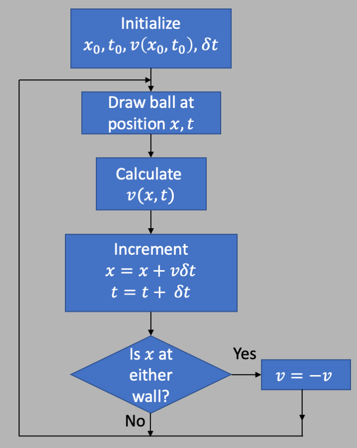
The prescription for coding this simulation would be something like the following diagram. We start with an initial value for $x$ and $t$: $x=x_0, t=t_0$. Then for each iteration, we calculate the velocity $v(x,t)$, then use that velocity and equation $\ref{master}$ to swim from this position to some new position. Then iterate. This works well as long as $v$ does not change "very much" over the interval $\dt$.
The pseudo-code would look something like this:
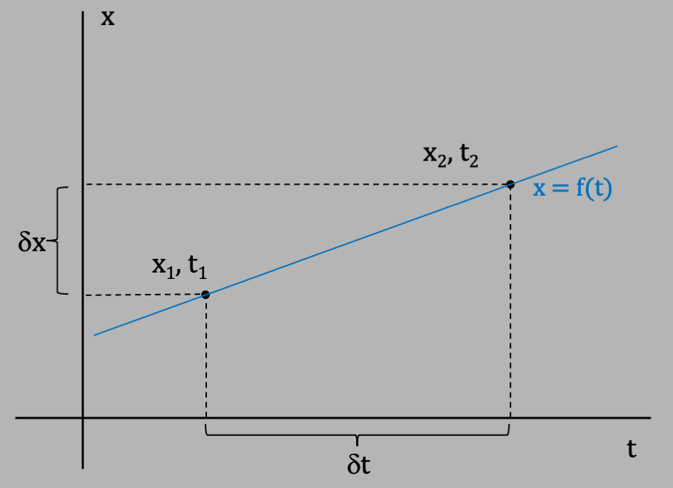
What we are doing here is can be represented graphically as in the following diagram where we are plotting $x$ vs $t$. The blue curve is the "true" curve of $x=f(t)$, and in this case where the ball is bouncing linearly off the walls, the velocity is constant so the blue curve is a straight line.
As discussed above, the Euler method is a simple linearization for solving an ordinary differential equation, and by "solving" we mean finding a way to go from $x(t_1)$ to $x(t_2)$, or more generally, $x(t)\to x(t+\dt)$. In general, say we know $$\dot x \equiv \frac{dx}{dt} = f(x,t)\nonumber$$ where the function $f(x,t)$ is some known function. In general, we know that $$\frac{dx}{dt} = \lim_{\dt\to 0}\frac{\dx}{\dt}\nonumber$$ where $\dx = x(t+\dt) - x(t)$. The approximation we are making is that for a sufficiently small $\dt$: $$\frac{dx}{dt} = \frac{\dx}{\dt} = f(x,t)\nonumber$$ which we can rewrite as $$x(t+\dt) = x(t) + f(x,t)\cdot\dt\nonumber$$ Sometimes, however, our differential equation is something like this where we start with the 2nd derivative, like in Newton's law: $$\frac{d^2x}{dt^2} = g(x,t)\nonumber$$ For this second derivative ODE, we apply Euler's method by defining $$v = \frac{dx}{dt}\nonumber$$ which means our differential equation becomes $$\frac{dv}{dt} = g(x,t)\nonumber$$ which is solved by $$v(t+\dt) = v(t) + g(x,t)\cdot\dt\nonumber$$ This gives us the 2 Euler equations: $$x(t+\dt) = x(t) + \dot x(x,t)\cdot\dt\label{eulerx1}$$ $$\dot x(t+\dt) = \dot x(t) + \ddot x(x,t)\cdot\dt\label{eulerv1}$$ where $\dot x = v(x,t)$ and $\ddot x = g(x,t)$. These 2 equations can also be written in a less obscure form: $$x(t+\dt) = x(t) + v(x,t)\cdot\dt\label{eulerx}$$ $$v(t+\dt) = v(t) + g(x,t)\cdot\dt\label{eulerv}$$ These equations tell us how to swim both the position, and the velocity, from one point to another over an interval $\dt$.
Let's take the simple example of projectile motion in a constant gravity field ("ballistic" motion, where you start with an initial energy and let it fly). Here the vertical acceleration is constant, so that $\ddot y = -g$ ($y$ measured positive up, acceleration is down and constant with value $g = 9.8m/s^2$), with initial conditions $y(0) = 0$ (start from the ground) and $\dot y(0) = v_0$. (We are ignoring the horizontal motion for now, but it's pretty easy since there is no horizontal acceleration.)
This motion is pretty easy to integrate, and we know the real (analytic) answer: $$\dot y(t) = v_0 - gt\label{eq3}$$ $$y(t) = v_0 t - \half g t^2\label{eq4}$$ The energy will be given by $E = \half m\dot y^2 + mgy$, and since energy is conserved and the initial energy is $E_0 = \half mv_0^2$, we should be able to verify this directly:
$$\begin{align} E & = \half m\dot y^2 + mgy \nonumber \\ & = \half m(v_0-gt)^2 + mg(v_0t-\half gt^2) \nonumber \\ & = \half mv_0^2-mgv_0t+\half mg^2t^2 + mgv_0t-\half mg^2t^2 \nonumber \\ & = \half mv_0^2\nonumber \\ \end{align}\nonumber$$ As expected!
But let's pretend we don't know how to integrate $\ddot y=-g$, and instead solve it numerically.
So if we start with $y(0)=0$ at $t=0$, and use equations (\ref{eulerx1}) and (\ref{eulerv1}), we would have after the $1^{st}$ iteration at time $\dt$: $$\begin{align} \dot y(\dt) & = \dot y(0) + \ddot y(0)\cdot\dt \nonumber \\ & = v_0 - g\dt\label{eq5} \\ y(\dt) & = y(0) + \dot y(0)\cdot\dt \nonumber \\ &= v_0\dt\label{eq6}\end{align}$$ We can calculate how far off this approximation is from the correct calculation we get from directly integrating $\ddot y=-g$, but we can also see it by calculating the energy after a time $\dt$: $$\begin{align} E(\dt) & = \half m\dot y^2 + mgy \nonumber \\ & = \half m(v_0-g\dt)^2 + mgv_0\dt \nonumber \\ & = \half mv_0^2-mgv_0\dt+\half mg^2\dt^2 + mgv_0\dt \nonumber \\ & = \half mv_0^2 + \half mg^2\dt^2\nonumber\end{align}\nonumber$$ We can see that this is off by an amount $\half mg^2\dt^2$ (2nd term in the last equation), which is also the amount that equation (\ref{eq6}) differs from equation (\ref{eq4}).
Taking another step in $\dt$ we get: $$\begin{align} \dot y(2\dt) & = \dot y(\dt) + \ddot y(\dt)\cdot\dt \nonumber \\ & = v_0 - g(2\dt) \nonumber \\ y(2\dt) & = y(\dt) + \dot y(\dt)\cdot\dt \nonumber \\ & = v_0(2\dt)-\frac{1}{4}g(2\dt)^2\nonumber \end{align}\nonumber$$ Again we see that the equation for $y(2\dt)$ is off,this time by an amount $\frac{1}{4}g(2\dt)^2$. When we calculate the energy we get $$\begin{align} E(2\dt) & =\half mv_0^2 + mg^2\dt^2 \nonumber \\ & = \half mv_0^2 + \frac{1}{2^2}mg^2(2\dt)^2\nonumber\end{align}\nonumber$$ For $3\dt$, we get $$\begin{align} \dot y(3\dt) & = \dot y(2\dt) + \ddot y(2\dt)\cdot\dt \nonumber \\ & = v_0 - g(3\dt)\nonumber \\ y(3\dt) & = y(2\dt) + \dot y(2\dt)\cdot\dt \nonumber \\ & = v_0(3\dt)-\frac{1}{3^2}g(3\dt)^2\nonumber\end{align}\nonumber$$ and the energy is given by $$\begin{align} E(3\dt) & = \half mv_0^2 + \frac{3}{2}mg^2\dt^2 \nonumber \\ & = \half mv_0^2 + \frac{1}{6}mg^2(3\dt)^2\nonumber \end{align}\nonumber$$ You can see that the energy per step is diverging, getting further away from energy conservation by adding another $\frac {1}{2}mg^2\dt^2$ at every step. So the bottom line is that the Euler technique is not so good - it violates energy conservation! Except it violates is to second order in $\dt$, so if you make $\dt$ small, you are still wrong, but only a little bit.
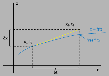
One obvious variation in the Euler technique is to use the slope at the end of the interval instead of at the beginning (aka "Euler-Cromer") as in the following figure:
The equations below show this explicitly: $$\dot y(t+\dt) = \dot y(t) + f(y(t+\dt),t+\dt)\cdot \dt\nonumber$$ $$y(t+\dt) = y(t) + \dot y(y(t+\dt),t+\dt)\cdot\dt\nonumber$$ Since just like in the above Euler case $f(y,t) = -g$ (constant gravity), then the 2 equations are: $$\dot y(t+\dt) = \dot y(t) - g\cdot \dt\label{eq7}$$ $$y(t+\dt) = y(t) + \dot y(y(t+\dt),t+\dt)\cdot\dt\label{eq8}$$ Starting at $t=0$, with $y(0)=0$ and $\dot y(0)=v_0$, after a time $\dt$ the equations become: $$\dot y(t+\dt) = \dot y(t) - g\cdot \dt\nonumber$$ $$y(t+\dt) = y(t) + \dot y(\dt)\cdot\dt\nonumber$$ This approximation is also imperfect, since as shown in the figure above, the slope at the end of the interval overestimates the average slope over the interval, and as you would expect, the value of $y(t+\dt)$ overestimates the true value. To illustrate, we can calculate the position and velocity after a time $\dt$: $$\begin{align} \dot y(\dt) &= \dot y(0) - g\cdot\dt\nonumber\\ &= v_0 - g\cdot\dt\nonumber \end{align}\nonumber$$ $$\begin{align} y(\dt) &= y(0) + \dot y(\dt)\cdot\dt\nonumber\\ &= (v_0 - g\dt)\cdot\dt\nonumber\\ &= v_0\dt - g\dt^2\nonumber \end{align}\nonumber$$ This gives the same answer for $\dot y(\dt)$ as with the straight Euler method, but differs in $y(\dt)$ by an amount $-g\dt^2$ (see equation $\ref{eq5}$ and $\ref{eq6}$).
The energy after time $\dt$ will be $$\begin{align} E(\dt) & = \half m\dot y^2 + mgy \nonumber \\ & = \half m(v_0-g\dt)^2 + mg(v_0-g\dt)\dt \nonumber \\ & = \half mv_0^2-mgv_0\dt+\half mg^2\dt^2 + mgv_0\dt - mg^2\dt^2 \nonumber \\ & = \half mv_0^2 - \half mg^2\dt^2\nonumber\end{align}\nonumber$$ And as above for the straight Euler case, energy is not conserved, and here instead of there being an extra $+\half mg^2\dt^2$, there's an extra $-\half mg^2\dt^2$.
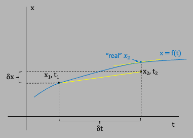
The Euler method uses the slope at $x_1,t_1$, and the Euler-Cromer uses the slope at $x_2,t_2$, to swim the position from $x_1,t_1$ to $x_2,t_2$. If the velocity is changing between these points in a smooth and regular way, then one of these methods will underestimate where $x_2$ should be and the other will overestimate. The logical thing to do is to consider using the value of the slope at the midpoint of the interval, $\dot x(t+\half \dt)$, as a better approximation to the average slope over the interval.
First, we can define $t_h = t+\half\dt$ as the time halfway between $t$ and $t+\dt$. Then we can define $x_h = x(t_h)$ and $\dot x_h = x(t_h)$. This will be a 2 step process, because to find $x_h$ and $\dot x_h$, we will use the Euler method to swim $x$ and $\dot x$ from $t$ to $t+\half\dt$, and use those values to swim $x$ and $\dot x$ from $x_1$ to $x_2$. This method is called "Runge-Kutta", aka RK (see this article in Wikipedia).
As always, we start with our initial conditions $x(0)=x_0$, $\dot x(0)=v_0$, and the differential equation $\ddot x = f(x,t)$. Then we calculate $x_h$ and $\dot x_h$ using Euler: $$x_h \equiv x(t+\half\dt) = x(t) + \dot x(x(t),t)\cdot\half\dt\nonumber$$ $$\dot x_h \equiv \dot x(t+\half\dt) = \dot x(t) + f(x(t),t)\cdot\half\dt\nonumber$$ Now we use $x_h$ and $\dot x_h$ to swim from $x_1$ to $x_2$. The equation for $x(t)$ becomes: $$\begin{align} x(t+\dt) & = x(t) + \dot x_h\cdot\dt\nonumber\\ & = x(t) + [\dot x(t) + f(t)\cdot\half\dt]\cdot\dt \nonumber\\ & = x(t) + \dot x(t)\cdot\dt + \half f(t)\cdot\dt^2\nonumber \end{align}\nonumber$$ The $\dt^2$ term shows that RK differs from Euler and Euler-Cromer in that it includes "higher order" terms. Because those higher order terms come in as $\dt^2$, we refer to this approximation as Runge-Kutta 2, or RK2 for short. We can expect it to be more accurate, which will be explored further below.
Note: it should be understood implicitly that $f(t)$ means the same thing as $f(x(t),t)$ if $g$ also depends on $x$. That is, when we write $\dot x(t)$ and $f(t)$ we mean a function where everything is evaluated at $t$, so if $f$ depends on $x$, then $f(t)$ means $f(x(t),t)$.
Now let's return to the example of throwing a ball up in the air, which is the more interesting part of ballistic or projectile motion. We use the coordinate $y$, and the acceleration is $\ddot y = f(y,t) = -g$ with initial conditions $y(0)=0$ and $\dot y(0)=v_0$. We first use Euler to calculate $y_h$ and $\dot y_h$, and start at t=0: $$\begin{align} y_h &\equiv y(t+\half\dt)\nonumber\\ &= y(0) + \dot y(0)\cdot\half\dt\nonumber\\ &= \half v_0\dt\nonumber \end{align}\nonumber$$ $$\begin{align} \dot y_h &\equiv \dot y(t+\half\dt)\nonumber\\ &= \dot y(0) + f(0)\cdot\half\dt\nonumber\\ &= v_0 - \half g\dt\nonumber \end{align}\nonumber$$ Then we use the above $y_h$ and $\dot y_h$ to swim $y(t)$ and $\dot y(t)$: $$\begin{align} y(\dt) &= y(0) + \dot y_h\dt\nonumber\\ &= 0 + [v_0 - \half g\dt]\dt\nonumber\\ &= v_0\dt - \half g\dt^2\nonumber\\ \end{align}\nonumber$$ $$\begin{align} \dot y(\dt) &= \dot y(0) + f(y_h,t_h)\dt\nonumber\\ &= v_0 - g\dt\nonumber\\ \end{align}\nonumber$$
The energy after a time $\dt$ will be given by: $$\begin{align} E(\dt) &= \half m\dot y(\dt)^2 + mgy(\dt)\nonumber \\ &= \half m[v_0-g\dt]^2 + mg[v_0\dt - \half g\dt^2]\nonumber \\ &= \half mv_0^2 - mv_0g\dt + \half mg^2\dt^2 + mg[v_0\dt - \half g\dt^2]\nonumber \\ &=\half mv_0^2\nonumber \end{align}\nonumber$$ which is not only closer to the correct answer than for Euler or Euler-Cromer, it is exactly the correct answer. Of course this is a special case: in fact, it's a special case for when the rate of change of the velocity is constant).
The next iteration takes the particle from time $t=\dt$ to time $t+\dt=2\dt$. The slope at the halfway point will be: $$\begin{align} \dot y_h \equiv \dot y(t+\half dt) &= \dot y(\dt) + f\cdot\half\dt\nonumber\\ &=v_0-g\dt - g\half\dt\nonumber\\ &= v_0 - \frac{3}{2}g\dt\nonumber \end{align}\nonumber$$ Note: we don't need to calculate $y_h$ for this case.
So the equations for the new $y$ and $\dot y$ are: $$\begin{align} y(t+\dt) \equiv y(2\dt) &= y(\dt)+\dot y_h\cdot\dt\nonumber\\ &=v_0\dt - \half g\dt^2 + (v_0- \frac{3}{2}g\dt)\cdot \dt\nonumber\\ &=2v_0\dt-2g\dt^2\nonumber \end{align}\nonumber$$ $$\begin{align} \dot y(t+\dt)\equiv \dot y(2\dt) &= \dot y(\dt) + f\cdot\dt\nonumber\\ &= v_0-g\dt-g\dt\nonumber\\ &= v_0-2g\dt\nonumber \end{align}\nonumber$$ The energy at this time will be $$\begin{align} E(2\dt) &= \half m\dot y(2\dt)^2 + mgy(2\dt)\nonumber \\ &=\half m[v_0-2g\dt]^2 + mg[2v_0\dt-2g\dt^2]\nonumber\\ &= \half m[v_0^2 -4v_0g\dt +4g^2\dt^2] + 2mv_0g\dt-2mg^2\dt^2\nonumber\\ &= \half mv_0^2\nonumber \end{align}\nonumber$$ As before, this shows that the RK approximation is exact. because is really a 2nd order correction to Euler. In fact, it's really nothing more than an expansion of $y(t+\dt)$ around $\dt$, keeping the terms up to order $\dt^2$. As you will see below, sometimes RK2 is all you need to do to get reasonable results. In the graph below, the solid line shows the exact solution of the parabolic path for a particle in a constant downward gravitational field. For comparision with the numerical integration, you can select using the radio buttons either: 1) the Euler technique (also known as the Explicit Euler); 2) the Cromer-Euler (also known as the Implicit Euler); or 3) the Runge-Kutta RK2. When you change the selection, remember to hit the Start button again. The Euler technique draws the path in blue circles, the Euler-Cromer in yellow, and the RK2 in red. Below that is a graph of the total energy, with arbitrary units that bring out the difference. You can easily see how the 3 techniques differ.
$|\vec {v_0}|=$
90
$\theta_0=$
65
Energy (arbitrary units):
To illustrate the limitations of the 3 method graphically, the figure below shows an arbitrary function $y=ax^3$ in blue. The starting and ending points are labeled $y(t)$ and $y(t+\dt)$ are drawn at times $t$ and $t+\dt$ respectively, drawn with solid black circles. The yellow line shows the slope calculated at some time, and drawn starting at the point $y(t)$. The radio buttons allow you to specify which of the 3 methods you want to use for the slope: $\dot y(t)$ for Euler, $\dot y(t+\dt)$ for Euler-Cromer, and $\dot y(t+\half\dt)$for Runge-Kutta. The value of $y(t+\dt)$ using one of the 3 approximations is drawn with an open blue circle. By changing the selection and hitting the "Redraw" button, you can see how close each of the approximations are to the true value (the one on the curve).
In the above example, we started with a simple (constant) 2nd derivative, $\ddot y = -g$. The 1st derivative would then be a function of time $t$, and so on for $y(t)$. However nature often throws us more difficult equations to integrate. The next one to study would be equations where the differentials are functions of external variables like $t$ and also of themselves, e.g. $\dot z = f(z(t),t)$.
For example, ballistic motion through the air should take into account air resistance. If the velocity is not too high, then the air resistance will be linear (against) the velocity: $$\vec F_{air} = -b\vec v\nonumber$$ We then have an equation of motion in $x$ (horizontal) and $y$ (vertical) given by: $$m\ddot x = -b\dot x\nonumber$$ $$m\ddot y = -mg - m\dot y\nonumber$$ To simplify, divide by $m$ and define $\tau\equiv m/b$ to get the equations: $$\ddot x = -\frac{\dot x}{\tau}\label{pmarx}$$ $$\ddot y = -g - \frac{\dot y}{\tau}\label{pmary}$$ These equations can be easily solved analytically to get: $$\begin{align} \dot x &=v_xe^{-t/\tau}\label{prx}\\ \dot y &= v_ye^{-t/\tau}+g\tau(1-e^{-t/\tau})\nonumber\\ x &=v_x\tau(1-e^{-t/\tau})\nonumber\\ y &= -g\tau t + (v_y-g\tau)\tau(1-e^{-t/\tau})\nonumber\\ \end{align}\nonumber$$ where at $t=0$, $x(0)=0$, $y(0)=0$, $\dot x(0)=v_x$, and $\dot y(0)=v_y$. As $t\to\infty$, $\dot x\to 0$ and $\dot y\to g\tau$, the terminal velocity. Similary for the horizontal position, as $\t\to\infty$, $x\to v_x\tau$, which means that the air resistance has eliminated any vertical velocity and the particle no longer goes any further along the horizontal.
Next we will show what happens when we apply the Euler method. Starting with equation $\ref{pmarx}$ and doing the horizontal $x$ coordinate first, we have: $$\begin{align} x(t+\dt) &= x(t) + \dot x(t)\cdot dt\nonumber\\ \dot x(t+\dt) &= \dot x(t) + \ddot x(t)\cdot dt\nonumber\\ &=\dot x(t) - \frac{\dot x(t)}{\tau}\cdot dt\nonumber\\ &=\dot x(t)[1-\frac{\dt}{\tau}]\label{preulerx} \end{align}$$ Starting at $t=0$ with the Euler method, and using the initial conditions $x(0) = 0$ and $\dot x(0)=v_x$, we have: $$\begin{align} x(\dt) &= x(0) + \dot x(0)\cdot \dt\nonumber\\ &= v_x\dt\nonumber\\ \dot x(\dt) &= \dot x(0)[1-\frac{\dt}{\tau}]\nonumber\\ &= v_x[1-\frac{\dt}{\tau}]\nonumber\\ \end{align}\nonumber\\$$ As you can clearly see, the Euler method for the horizontal velocity (equation $\ref{preulerx}$) is equivalent to an expansion of the analytical solution (equation $\ref{prx}$) keeping only the first order term, since the expansion for $e^{-t/\tau}$ is $$e^{-t/\tau} = 1 - \frac{t}{\tau} + \half \big(\frac{t}{\tau}\big)^2 +-...\nonumber$$ The Euler-Cromer gives something similar, still first order in $t/\tau$.
The RK method is next. As usual, we define $t_h = t + \half\dt$. For motion along the horizontal, we have the same differential equation as in $\ref{pmarx}$. We use the Euler method to find $\dot x_h$ (we don't need $x_h$ here): $$\begin{align} \dot x_h &= \dot x(t) + \ddot x(t)\cdot\half\dt\nonumber\\ &= \dot x(t) - \frac{\dot x(t)}{\tau}\half\dt\nonumber\\ &= \dot x(t)[1-\frac{\dt}{2\tau}]\nonumber \end{align}\nonumber\\$$ Which gives $$\ddot x(t_h) = -\frac{\dot x(t_h)}{\tau}=-\dot x(t)\frac{1-\dt/2\tau}{\tau}\nonumber$$ The expansion for $x(t+\dt)$ and $\dot x(t+\dt)$ is given by $$\begin{align} x(t+\dt) &= x(t) + \dot x(t_h)\dt\nonumber\\ &= x(t) -\dot x(t)\dt\frac{1-\dt/2\tau}{\tau}\nonumber\\ \dot x(t+\dt)&= \dot x(t) + \ddot x(t_h)\dt\nonumber\\ &= \dot x(t) - \dt\frac{\dot x(t)}{\tau}[1-\frac{\dt}{2\tau}]\nonumber\\ &= \dot x(t)\big[1-\frac{\dt}{\tau}+\frac{\dt^2}{2\tau^2}\big]\nonumber \end{align}\nonumber$$ And again, here you see explicitly how RK includes 2nd order terms in $\dt/\tau$ for the velocity.
For the vertical component of motion, we have the same differential equation as in $\ref{pmary}$. So we first form $$\ddot y(t_h) = -g - \dot y(t_h)\nonumber$$ and calculate $\dot y(t_h$ as $$\begin{align} \dot y(t_h) = \dot y(t+\half\dt) &= \dot y(t) + \ddot y(t)\half\dt\nonumber\\ &=\dot y(t) - \half\dt\big(g+\frac{\dot y(t)}{\tau}\big)\nonumber\\ &= \dot y(t)\big[1-\frac{\dt}{2\tau} \big]-\half g\dt\nonumber \end{align}\nonumber$$ This gives the equations for $y(t+\dt)$ and $\dot y(t+\dt)$: $$\begin{align} y(t+\dt) &= y(t) + \dot y(t_h)\dt\nonumber\\ &= y(t) + \dot y(t)\dt\big(1-\frac{\dt}{2\tau}\big)\nonumber\\ \dot y(t+\dt) &= \dot y(t) + \ddot y(t_h)\dt\nonumber\\ &= \dot y(t) - (g+\frac{\dot y(t_h)}{\tau})\dt\nonumber\\ &= \dot y(t) - (g+\frac{1}{\tau}\dot y(t)[1-\frac{\dt}{2\tau}]-\half g\dt)\dt\nonumber\\ &=\dot y(t)\big[1-\frac{\dt}{\tau}+\frac{\dt^2}{2\tau^2}\big] - g\dt\big[1 - \frac{\dt}{2\tau}\big]\nonumber \end{align}\nonumber$$
RK works rather well, as you can see from the interactive figure below. You can use the sliders to change the initial conditions, the "Rescale" will allow the curve to fit in the window, and you can toggle the air resistance on and off (on will draw a black curve, off will draw a white one). The solid line is the analytic solution, the points are from using the various methods for simulation.
| $k/m$ | 0.1 | |
| $|\vec {v_0}|$ | 130 | |
| $\theta_0$ | 60 | |
| Rescale | 1 |

We will first use Newton's law to calculate the force components, but then switch to Lagrangians, to warm you up for the inevitable consideration of the double pendulum.
We take the coordinate origin $(0,0)$ to be the point where the pendulum ball (with mass $m$) is completely vertical with no motion, equivalent to $\phi=0$. The coordinates $(x,y)$ will be relative to that resting point.
The equations of motion are: $$\begin{align} \ddot x &= 0\nonumber\\ \ddot y &= -g\nonumber\\ \end{align}\nonumber$$ At $t=0$, we raise the pendulum to some angle $\phi_0$ and let it go. At that point $x(0)=L\sin\phi_0$, $\dot x(0)=0$, $y(0)=L - L\cos\phi_0$, and $\dot y(0)=0$.
Here $(x,y)$ are constrained by the pendulum such that $x^2+y^2=L^2$, so there's really only 1 free coordinate, the angle $\phi$. So we will instead solve for $\phi(t)$, which means that instead of using Newton's law of forces, we will use the angular equivalent, which involves moment of inertia and angular acceleration.
The moment of inertia $I$ measures the extent of a object, relative to a pivot point. Here the pivot point is fixed, and the object is at a fixed distance. Formally, $I$ is calculated as the integral of the mass density $\rho$ over the volume, weighted by the distance squared from the pivot: $$I = \int \rho(r)|r|^2dV\nonumber$$ For the pendulum, since all the mass is at a fixed distance $r=L$, the integral gives just the mass $m$, and $I$ simplifies to $$I = mL^2\label{moi}$$ The equation for circular motion equates the angular acceleration $\ddot\phi$ to the torque about the pivot, $F\cdot L_\perp$, which gives: $$I\ddot\phi = F\cdot L_\perp\nonumber$$ $L_\perp$ is the perpendicular distance between the location of the mass and the force of gravity, which is given by $L_\perp=L\sin\phi$, and since the force $F$ is due to gravity, $F=-mg$. This gives us the equation of motion $$I\ddot\phi = -mgL\sin\phi\nonumber$$ or equivalently: $$\ddot\phi + \frac{g}{L}\sin\phi=0\label{eqmphi}$$ As an aside, there's an alternate derivation using Lagrangians. We can start with $$\begin{align} x &= L\sin\phi\nonumber\\ y &= L(1-\cos\phi)\nonumber \end{align}\nonumber$$ And differentiate to get $$\begin{align} \dot x &= L\dot\phi\cos\phi\nonumber\\ \dot y &= L\dot\phi\sin\phi\nonumber \end{align}\nonumber$$ and form the kinetic energy $$KE = \half mv^=\half m(\dot x^2+\dot y^2)=\half mL^2\dot\phi^2\nonumber$$ The potential energy due to gravity is just $$PE = mgy=mgL(1-\cos\phi)\nonumber$$ Combining, we form the Lagrangian $$\mathcal L=T-V=\half mL^2\dot\phi^2-mgL(1-\cos\phi)\label{lagr}$$ with equations of motion $$\frac{d}{dt}\frac{\partial \mathcal L}{\partial\dot\phi}-\frac{\partial\mathcal L}{\partial\phi}=0\label{leq}$$ with $$\frac{\partial\mathcal L}{\partial\phi}=-mgL\sin\phi\nonumber$$ $$\frac{\partial \mathcal L}{\partial\dot\phi}=mL^2\dot\phi\nonumber$$ and $$\frac{d}{dt}\frac{\partial \mathcal L}{\partial\dot\phi}= \frac{d}{dt}mL^2\dot\phi=mL^2\ddot\phi\nonumber$$ Then applying equation $\ref{leq}$ gives $$mL^2\ddot\phi+mgL\sin\phi=0\nonumber$$ or $$\ddot\phi + \omega_0^2\sin\phi=0\label{eqmotion}$$ where $$\omega_0^2\equiv \frac{g}{L}\nonumber$$ which is the same equation as derived above using Newton's laws for circular motion. This gives us the equation $$\ddot \phi=-\omega_0^2\sin\phi\label{pendulum}$$ which we will need below for the simulation.
The total energy of this system, which we will need later, is give by
$$E=T+V=\half mL^2\dot\phi^2+mgL(1-\cos\phi)\nonumber$$
At $t=0$, since $\dot\phi(0)=0$, the total energy is
$$E=T+V=mgL(1-\cos\phi)\label{totalE}$$
Pendulum and Euler Method
Next we form the equations to simulate using the Euler method:
$$\begin{align}
\phi(t+\dt)&=\phi(t)+\dot\phi(t)\dt\nonumber\\
\dot\phi(t+\dt)&=\dot\phi(t)+\ddot\phi(t)\dt\nonumber\\
&=\dot\phi(t)-\omega_0^2\sin\phi(t)\dt\nonumber
\end{align}\nonumber$$
And as before, when we write $\dot\phi(t)$ we mean $\dot\phi\big(\phi(t),t\big)$.
Starting from the initial conditions $t=0,\phi(0)=\phi_0,\dot\phi(0)=0$, after time $\dt$ we have: $$\begin{align} \phi(\dt) &= \phi(0)+\dot\phi(0)\dt\nonumber\\ &=\phi_0\nonumber\\ \dot\phi(\dt)&=\dot\phi(0)-\omega_0^2\sin\phi_0\dt\nonumber\\ &=-\omega_0^2\sin\phi_0\dt\nonumber \end{align}\nonumber$$ At the time $t=\dt$, the energy $E(\dt)$ is: $$\begin{align} E(\dt) &= \half mL^2\dot\phi^2(\dt)+mgL(1-\cos\phi(\dt))\nonumber\\ &= \half mL^2\big(-\omega_0^2\sin\phi_0\dt\big)^2+mgL(1-\cos\phi_0)\nonumber\\ &=\half mL^2(g/L)^2\dt^2\sin^2\phi_0+mgL(1-\cos\phi_0)\nonumber\\ &=\half mg^2\dt^2\sin^2\phi_0+mgL(1-\cos\phi_0)\nonumber\\ \end{align}\nonumber$$ This overestimates the correct energy $E=mgL(1-\cos\phi_0)$ by an amount proportional to $\dt^2$. To see how this evolves, let's calculate $\phi$ and $\dot\phi$ after the next interval of $\dt$: $$\begin{align} \phi(2\dt) &= \phi(\dt)+\dot\phi(\dt)\dt\nonumber\\ &=\phi_0-\big(\omega_0^2\sin\phi_0\dt\big)\dt \nonumber\\ &=\phi_0-\omega_0^2\sin\phi_0\dt^2 \nonumber\\ \dot\phi(2\dt)&=\dot\phi(\dt)-\big(\omega_0^2\sin\phi_0\big)\dt\nonumber\\ &=-2\omega_0^2\sin\phi_0\dt\nonumber \end{align}\nonumber$$ The energy $E(2\dt)$ is therefore $$\begin{align} E(2\dt) &= \half mL^2\dot\phi^2(2\dt)+mgL(1-\cos\phi(2\dt))\nonumber\\ &= \half mL^2\big(-2\omega_0^2\sin\phi_0\dt\big)^2+ mgL\big[1-\cos\big(\phi_0-\omega_0^2\dt^2\sin\phi0\big)\big]\nonumber\\ &=\half mg^2(2\dt\sin\phi_0)^2+ mgL\big[1-\cos\big(\phi_0-\omega_0^2\dt^2\sin\phi0\big)\big]\nonumber\\ \end{align}\nonumber$$ As you can see, this energy divergance is increasing over time.
Pendulum and Runge-Kutta Method
Using equation $\ref{pendulum}$ for the differential equation governing the motion of $\phi(t)$, we first form the halfway coordinates for Runge-Kutta $$\begin{align} \ddot\phi_h &\equiv -\omega_0^2\sin\theta(t+\half\dt)\nonumber\\ \phi_h&=\phi(t+\half\dt) = \phi(t)+\dot\phi(t)\half\dt\nonumber\\ \end{align}\nonumber$$ which gives $$\ddot\phi_h = -\omega_0^2\sin\big(\phi(t)+\half\dot\phi(t)\dt\big)\nonumber$$ Also, $$\begin{align} \dot\phi_h&\equiv\dot\phi(t+\half\dt) = \dot\phi(t)+\half\ddot\phi(t)\dt\nonumber\\ &=\dot\phi(t)-\half\omega_0^2\dt\sin\phi(t)\nonumber \end{align}\nonumber$$ Now we can use the RK method for a simulation. For $\phi(t+\dt)$: $$\begin{align} \phi(t+\dt) &= \phi(t) + \dot\phi_h\dt\nonumber\\ &=\phi(t) + \big[\dot\phi(t)-\half\omega_0^2\dt\sin\phi(t)\big]\dt\nonumber\\ &=\phi(t) + \dot\phi(t)\dt - \half\omega_0^2\dt^2\sin\phi(t)\nonumber \end{align}\nonumber$$ The first 2 terms on the right hand side are the same terms for the Euler method, which is linear in $\dt$, but the 2nd term is quadratic - $\dt^2$ - again telling us that the Runge-Kutta method is a higher order approximation in $\dt$. For $\dot\phi(t+\dt)$: $$\begin{align} \dot\phi(t+\dt) &= \dot\phi(t) + \ddot\phi_h\dt\nonumber\\ &=\dot\phi(t) - \omega_0^2\dt\sin\big[\phi(t)+\half\dot\phi(t)\dt\big]\nonumber \end{align}\nonumber$$ Using the same initial conditions as we used for the Euler method, after $t=0$ we have $$\begin{align} \phi(\dt)&=\phi(0)+\dot\phi(0)\dt- \half\omega_0^2\dt^2\sin\phi(0)\nonumber\\ &= \phi_0 - \half\omega_0^2\dt^2\sin\phi_0\nonumber\\ \dot\phi(\dt) &= \dot\phi(0) - \omega_0^2\dt\sin\big[\phi(0)+\half\dot\phi(0)\dt\big]\nonumber\\ &=-\omega_0^2\dt\sin\phi_0\nonumber \end{align}\nonumber$$ The energy at time $t=\dt$ will be: $$\begin{align} E(\dt) &=\half mL^2\dot\phi^2(\dt) + mgL(1-\cos\phi(\dt))\nonumber\\ &=\half mL^2\big[-\omega_0^2\dt\sin\phi_0\big]^2 + mgL\big[1-\cos\big(\phi_0-\half\omega_0^2\dt^2\sin\phi_0\big)\big]\nonumber\\ &=\half mg^2\dt^2\sin^2\phi_0 + mgL\big[1-\cos\big(\phi_0-\half\omega_0^2\dt^2\sin\phi_0\big)\big]\label{eedt}\\ \end{align}\nonumber$$ The 2nd part of the above equation has a complicated term in $\cos(\phi_0 - \delta)$ where $\delta$ is defined as $\delta\equiv \half\omega^2\dt^2\sin\phi_0$, which is proportional to the higher order term $\dt^2$. This term can be written as: $$\cos(\phi_0-\delta) = \cos\phi_0\cos\delta+\sin\phi_0\sin\delta\nonumber$$ Given that $\phi_0$ is constant and that we can make $\dt$ arbitrarily small, then $\phi_0\gt\gt\delta$ so we can use the approximation $\sin\delta\to\delta$ and $\cos\delta\to 1$, which gives us: $$\cos(\phi_0-\delta)\to\cos\phi_0 + \delta\sin\phi_0\nonumber$$ Substituting this into equation $\ref{eedt}$ gives: $$\begin{align} E(\dt) &=\half mg^2\dt^2\sin^2\phi_0 + mgL\big[1-\cos\big(\phi_0-\half\omega_0^2\dt^2\sin\phi_0\big)\big]\nonumber\\ &\to \half mg^2\dt^2\sin^2\phi_0 + mgL\big[1-\cos\phi_0 - \delta\sin\phi_0\big]\nonumber\\ &= \half mg^2\dt^2\sin^2\phi_0 + mgL\big[1-\cos\phi_0 - \half\omega_0^2\dt^2\sin\phi_0\sin\phi_0\big]\nonumber\\ &=mgL(1-\cos\phi_0)\nonumber \end{align}\nonumber$$ which gives the exactly correct analytic answer. Evidently, for a pendulum, Runge-Kutta is as high an order as you need to go.
Here you can see clearly the accuracy of the RK2 method comes from the fact that it contains terms of order $\dt^2$, as pointed out above. This is basically just saying that when you do a Taylor expansion of the integral you are trying to calculate numerically, with RK2 you are keeping higher order terms.
A comment about 4th order Runge-Kutta (aka RK4): this involves breaking up the interval into 4 segments instead of 2 with RK2. It is definitely more accurate, however whether it's worthwhile depends on the problem being tackled. One can easily get a similar accuracy with RK2 by just making the interval $\dt$ smaller, approaching the same accuracy for RK4. However if the process you are simulating is taking lots of CPU time, then RK4 might get you there faster.
In the simulation below, we use blue for the Euler method, yellow for the Euler-Cromer, and red for the RK2 method. The first box below the pendulum shows the energy (somewhat arbitrary units) for the 3 different methodds. The Euler method violates energy conservation maximally and diverges, the Euler-Cromer violates it but not so bad, and it oscillates. The RK2 method is quite good, you can't even see the energy violation without a large scale factor like 100 (try it!).
| $\dt$ | 0.25 | |
| Time between calls | 5 |
All rights reserved. No part of this publication may be reproduced, distributed, or transmitted in any form or by any means, including photocopying, recording, or other electronic or mechanical methods, without the prior written permission of the publisher, except in the case of brief quotations embodied in critical reviews and certain other noncommercial uses permitted by copyright law.