University of Maryland Physics Education Research Group
 |
Physics Software from the UMd PERG:
Pendulum -- Simulation for a Damped, Driven Pendulum |
I. D. Johnston, M. A. Oldfield, University of Sydney
E. F. Redish, University of Maryland
Download File (36 KB)
Brief description
This program solves and displays the motion of a pendulum. Graphs of the angle, angular velocity, and energies (kinetic, potential, and total) are displayed linked in time. One can also view the phase plane and an animation of the motion. Damping and forcing motions can also be set. Parameters can be adjusted and values read off the graphs.
Pedagogical utility
This program gives a student an early example of a non-linear force law. The student can compare the linear approximation (done analytically or using the program HarmOsc) to the exact solution. The dependence of the period on amplitude may be investigated as may the chaotic result of including oscillatory forcing.
Appropriate for
- Physics 142
- Physics 262
- Physics 272
and possibly in part for Physics 117 and 122 (not tested)
Screen views
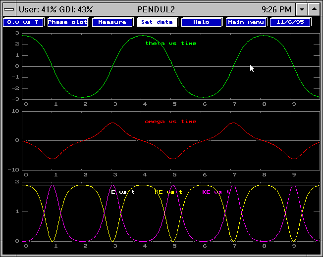
Fig. 1: The display of angular position, velocity, and energies
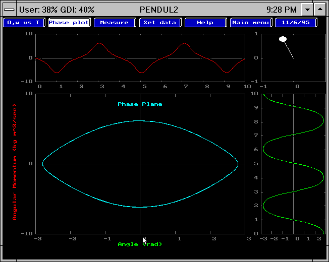
Fig. 2: The display of the phase plane and the animation.
Availability
The code may be downloaded by clicking here.
(36K)
The file is a zip file. Unpack it using WinZip.
You will then find the following files in your directory:
- egavga.bgi (6K) -- the graphics driver for the file
- pulses.exe (64K) -- The main executable
Technical information
The program solves the equation of motion using a fourth-order Runge-Kutta method.
Associated materials
There is a long homework problem (equivalent to about two typical end-of-chapter problems) using this program available from E. F. Redish.
Contact person
E. F. Redish, University of Maryland, College Park, MD 20742;
phone: 301-405-6120, fax: 301-314-9531, e-mail: redish@physics.umd.edu
Program help
The menu items on the menu you see first (the main menu) do the following things:
- SET DATA :
- Allows you to set the parameters of the problem
- GRAPHS:
- Plots the graphs.
- OPTIONS:
- Allows you to change what is displayed or the solution method.
- HELP:
- Brings up a screen describing what the menu items do.
- QUIT:
- Ends the program.
Select SET DATA and press < enter > . The first time you do this you will see the option screen. It allows you to
- change the numerical method by which the equations are solved
- change the kind of damping force used
- slow down the display by inserting a time delay.
If you press < enter > from the options screen, you will now see the data-entry screen. The parameters of the problem are shown on this screen. The numbers the program is currently using are shown in the black boxes. You can change any of them by typing over the numbers that are there. Use the arrow keys to change your position on the data-entry screen. Press < enter > to accept this data.
There are now three graph windows that display the anglle, angular velocity, and energies (kinetic, potential, and total) as a function of time.
Notice that the menu has changed. This is the graph menu. The entries are selected and activated in the same way as those of the main menu, by highlighting them with the arrow keys and pressing < enter > . The entries do the following things:
- X, V, vs. T
- Redraws the graphs.
- PHASE PLOT
- Plots X vs. V
- VALUES:
- Lets you to read a point off a graph using the mouse cursor.
- SET DATA
- Brings you back to the data entry screen
- HELP:
- Brings up a screen describing what the menu items do.
- MAIN MENU:
- Returns to the main menu.
If you select PHASE PLOT from the graph menu, the program will display three graphs and an animation of the mass's motion. The large graph in the center will display a plot of the position vs. the velocity. The two side graphs will display the position and the velocity as a function of time. The plotting of the graphs and the motion of the animation are all synchronized.