Teaching Physics with the Physics Suite
Edward F. Redish
Home | Action Research Kit| Sample Problems | Resources | Product Information
Problems Sorted by Type | Problems Sorted by Subject | Problems Sorted by Chapter in UP
|
Teaching Physics with the Physics Suite Edward F. Redish Home | Action Research Kit| Sample Problems | Resources | Product Information | |
Problems Sorted by Type | Problems Sorted by Subject | Problems Sorted by Chapter in UP |
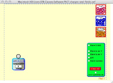
| In this problem,
you will use the simulation "Charges and Fields" from
the University of Colorado's PhET group. This program allows you
to explore the electric field and electrostatic potential produced
by charges that you can place on the screen. The opening screen
is shown at the right.
Note that on the opening screen, you have (at the top right of the screen) boxes of (red) positive and (blue) negative charges (1 nC each) and a box of E-Field Sensors (test charges that are so small they don't affect any of the other charges). Explore the program by grabbing some red and blue charges from the box with your mouse, placing them on the screen, and exploring the field they produce with one or more E-Field sensors. (The sensors don't show anything until you drop them, but after you do, they show an arrow representing the E-Field and then, as you move them around, the continue to show the E-Field.) |
 |
To get rid of sensors or charges, put them back in their boxes.
You can also turn on a grid for convenience of placing charges and you can turn on a display of E-Fields at a set of grid points.
A. How do the representations of the E-Field using the E-Field sensor and the "Show E-Field" box differ? Which do you prefer and why?
B. When you turn on the grid, it shows a distance scale (2 large grid boxes = 1 m). The electric field arrows on the E-field sensors are to a different scale since you don't measure E-field in meters but in Newtons/Coulomb. Can you figure out what grid scale the program uses for the E-field arrow on the E-field sensor? If you can, do it. If you can't, explain why not.
You can also use the potential meter (shown at the lower left of the screen above) to measure the potential (in Volts) at the point under the cross at the top of the meter. It will also draw the equipotential surface through that point. (At least the part of the surface that interacts the plane that it is showing.)
C. Construct equipotential surfaces for the following 3 configurations: a point charge, a dipole, and a quadrupole (four charges of equal magnitude on the four corners of a square, with the charges on adjacent corners having opposite sign). Draw enough equipotentials to get an idea of the way they behave. Choose values so that the values of the potential on your lines are equally spaced (e.g., draw equipotentials for potential values of 10, 9.5, 9, 8.5, 8, etc.). Sketch a careful graph of the potential along the x-axis. (Take this to run through the center of each configuration but orient your dipole and quadrupole so that the x-axis does not run through a charge. It will, of course, do so for a single charge.)
D. When creating a program such as this that only displays information about E-fields and potentials in a plane, one has a choice to make. One can say, "We live in a 3-D world, but I can only display 2-D of it. I'll just restrict myself to 2 of those 3 dimensions." Or one can say, "Let's pretend that we actually live in a 2-D world and the charges cannot even in principle move out of the plane of the computer screen." It turns out that if one makes the second assumption, surprisingly the electric field from a point charge does not fall of like 1/r2; it only falls off like 1/r.* Which choice did the designer of this program make? Explain your decision with quantitative observations.
* It's hard to see why this is the case if one only knows Coulomb's law. Why not just use the same law in 2-D? But Coulomb's law in 3-D arises from a set of principles called field equations that describe not only electric forces but magnetic fields, the interaction of electric and magnetic fields, and their behavior and propagation in empty space. If these equations are solved in 2-D instead of 3-D one gets the result quoted.
Page last modified April 16, 2009: E59