A Thinking Person's Guide to Programmable Logic
(End of Page)
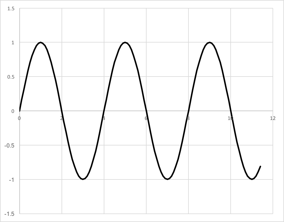
Imagine you are doing an experiment that is looking at some incoming time varying voltage signal, which might look like this:
Now imagine that the physics you want to get to involves understanding the power spectrum as a function of frequency for the incoming wave, so you will want to execute a Fourier transform on the incoming signal. Normally, what you might do is to build electronics that uses an ADC to digitize the incoming signal at some time interval that is small compared to the period of the incoming wave. So if you took some data over a time period of several wavelengths, you would see a series voltage measurements at successive time intervals, and if you made a plot of the voltage at the given times you might see something like this:
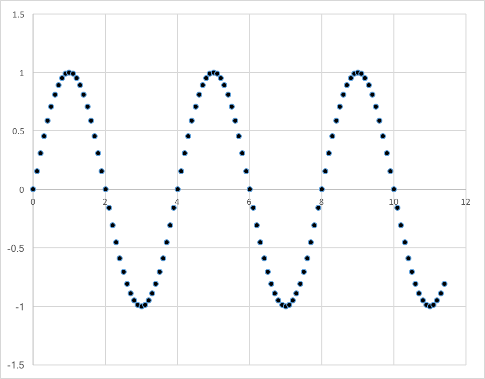
What you might want to do is use this data to measure the frequency of the incoming signal. So far this is pretty easy - if you applied a simple fourier transform to this data, you would get the right value. The only caveat is that the time between measurements is small compared to the period of the incoming signal.
In the real world, the incoming signals will be subject to two important effects: noise, and efficiency. By "noise", what is meant is that what is measured will be the sum (remember the principle of superposition) of a signal, plus stuff that is not only independent to the signal, but random in nature. By "efficiency", what is meant is that there is some probability different from 1 that given a signal, you actually see it. This probability can be near 0 (inefficient) or near 1 (completely efficient).
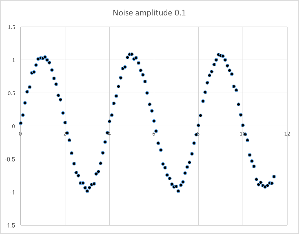
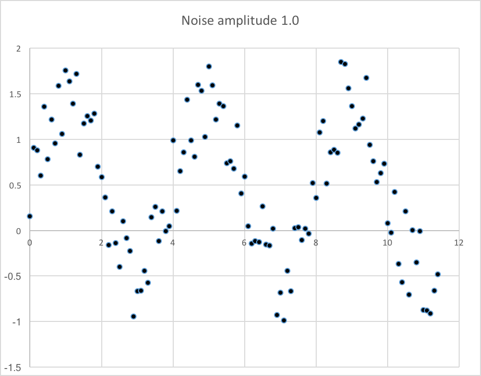
First, the noise. Imagine that the signal you are measuring is some waveform with sopme frequency $f$ and amplitude $A$ represented by $$S(t) = A\sin\omega t\nonumber$$ The noise can be distributed uniformly in some interval. If the interval $A_N$ was small compared to the amplitude of the signal $A$, say $A_N = 0.1A$, then the combined signal would look like this:
Now let's consider efficiency. By efficiency, we mean that the signal you are trying to detect might, or might not, be present. For instance, imagine you have a telescope and you are pointing it at a very distant galaxy, and imagine the telescope has a very small area of view, so that it's looking only at that particular galaxy. That galaxy is so far away that any photon emitted would have to be exquisitely pointed at the earth in order to make it. Anything inbetween earth and the galaxy that deflects the photon by even the smallest amount will cause the photon to miss the telescope. So if the galaxy were to emit a continuous stream of photons, each one would have a finite probability of being detected, which means that the data you collect at some time interval might be data + noise, or it might be only noise, because the data has a finiite detection efficiency.
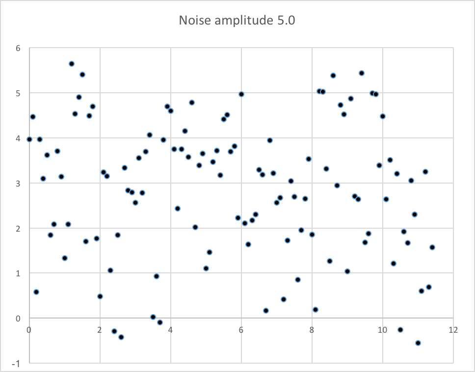
In the plot below, you can see an incoming sine wave after digitization. You can use the sliders to change the noise level (random noise) and the detection efficiency, and see how the incoming signal begins to look less like a periodic waveform and more like random noise.
Efficiency=%
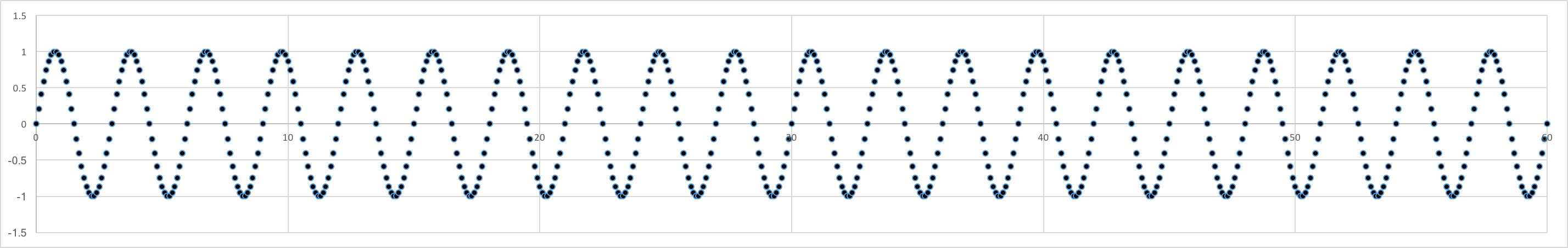
The challenge is to dig the real signal out of the noise. To understand how to do this, the following picture shows many periods of the incoming wave:
We sample at a constant rate $\delta t$, but we do not know the period of the wave. To integrate, we capture $N_{int}$ samples in a row, and add then to the previous $N_{int}$ samples, again and again. In the plot below, we choose a random value for $\delta t$ and the period $T$, and an initial value for $N_{int}$, and integrate (sum) 100 chunks. Using the slider you can vary $N_{int}$, and clearly see how if we guess right all of the waves will add up constructively. The condition for constructive interference will be $N_{int}\cdot\delta t = n\cdot T$ where $n$ is an integer.
Integration works, but mostly if we guess right. If we guess wrong, you can still see an oscillation, however if you add noise and inefficiency on top of this, you would have no chance. We need something smarter.
One way to overcome the above problem (not knowing the optimal period of integration) is to correlate the incoming signal with itself at various delays. This kind of self-correlation is also known For instance, imagine you have an incoming function $S(t_1) = A\sin\omega t_1$ ($\omega = 2\pi/T$), you produce a delayed version $S(t_2) = A\sin\omega t_2$, and add them together. The resulting waveform will be $$S(t_1) + S(t_2) = 2A\cos(\frac{\tau}{2})\sin(\bar{t})\nonumber$$ where $\tau = t_1-t_2$ (often referred to as the "beat period") and $\bar{t} = \half(t_1+t_2)$ is the average of the two.
Clearly, if you delay the incoming wave by a time $\tau$ which is a multiple of the period $T$, the waves will add constructively. This is demonstrated in the above plot where you vary the integration time (effectively, the delay between the incoming waves) and see enhancement at values of $\tau = nT$ ($n$ integer).
This is the idea behind what is called "autocorrelation", where instead of integrating the entire waveform "chunk" (summing over values in the same bin), you correlate the incoming data with a set of data each delayed by a linearly increasing amount. Autocorrelation is the same as a "convolution", defined mathematically as: $$(f\circ g)(t) = \int_0^t f(t-\tau)g(\tau)d\tau\nonumber$$
However in our case, the two functions are the same (hence the "auto" in autocorrelation), and we will correlate a finite chunk, each piece at a different delay, with the incoming signal. Note that a fundamental thing about convolution (and autocorrelation) is that we are first multiplying pieces of the waveform together, and then adding (integrating). The main idea is that we don't know what the period is of the incoming wave, but it has to be such that some piece of the delayed waveform will be at the same phase as the incoming piece, so that when multipled together and added, it will add up to something significant.
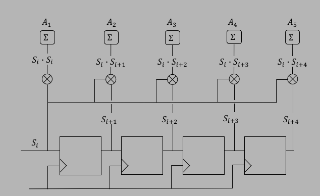
In the FPGA, the autocorrelator looks like the following figure. In this implementation, the incoming signal $S_i = S(t_i)$ is a single bit, and there are 5 states of correlation. The clock frequency for the shift register is $1/delta t$, and each time there's a new reading, you shift again, so that after $N$ readings, $S_i$ is shifted all of the way through. After each shift, the next data point $S_i$ is multiplied by the shifted value ($S_{i+1}, S_{i+2}$, etc) forming $S_i\cdot S_{i+1}$ and so on. Then we keep summing at each shift stage to produce $A_k, k=1,N$.
The controls below allow you to simulate an incoming signal (or two incoming signals), you can set the amplitude and period of each, and add noise and efficiency. You can think of the amplitude as being in arbitrary length units, and the period in seconds. The system will use a 10Hz clock, or a clock with a 0.1s period, producing a digital (discretized) signal every 0.1s. You can also set an arbitrary phase, in degrees, between the two signals.
The number of bits in the ADC is programmable, initially set to 0. You can change the number of bits to as large as 10, which means that the ADC will produce 1024 different values, which means each bit will mean 1/1024 of the total amplitude. The default is 1 bit, and it might be surprising to find that for many purposes, 1 bit is enough to see the relevant spectrum. You can also turn on noise with an amplitude (same units) and you can employ an efficiency for the incoming signal (not the noise, of course). Hit the Start button to start, and you can change things dynamically but it is usually better to hit Reset (equivalent to Stop with a reset of the spectrum sums). The simulation is pretty good at showing the power of autocorrelation!
| Function 1 | A1: | |
| T1: | ||
| Function 2 | A2: | |
| T2: | ||
| $\Delta\phi$ (deg) |
| Noise Amplitude | ||
| Efficiency | ||
| ADC Bits |
Try setting the controls for 1 function, put in an equal amplitude for noise, and some inefficiency (say 50%). Keep the ADC to 1 bit and hit start. If you run it for 1000 or greater inputs, you will see something like the following. Clearly this is a pretty good filter even with only 1 bit. Note that in the work of CD players, 1 bit is (or was, when they were still being made) the norm, because 1 bit is good enough!
The last button on the right is labeled "Fourier". When you hit this button, it will execute a discrete fourier transform, and display the coefficients for the cosine basis functions. You can see a few things clearly here:
We will build on the previous voltmeter2 project to instantiate the XADC and the serial I/O, and add the autocorrelator. For this project, we will input a signal that will come from some kind of audio source, like a microphone or an MP3 player, which means that the signal will be in the audio range ($0\to\sim 20$kHz). These signals are typically digitized at 44100Hz, to be able to be sensitive up to the $\sim 20$kHz signals (the Nyquist frequency, see the section on fourier analysis). Remember, the XADC takes the clock, divides it by the clock divider parameter, and then divides that by 26 for the sampling time. So when we ran the voltmeter2, we started with a $50$MHz clock, divided by 2 to get $25$MHz, then divided by 26 to get $0.961$kHz digitization. It would be great if we could run the XADC at $44.1$kHz, but when we run it in "Continuous Mode" (like we did for voltmeter_continuous), the minimum clock frequency (DCLK) is $8$MHz and the minimum ADC conversion rate after dividing is $154$kHz ($8$MHz, x2 divider, x26 divider for the digitation equals $153.846$kHz). Since we are starting with a $100$MHz system clock, we will divide it by 8 to produce a $12.5$MHz DCLK, and set the "ADC Conversion Rate" to $160.26$kHz. That will produce a clock divider value of 3. This gives us lots of spare time for state machines and combinatorial logic. Digitizing at $160.26$kHz is effectively oversampling. If our target digitization is $44.1$kHz, then $162.26$kHz divided by 4 is $40.065$kHz, close enough to $44.1$kHz so we could either just keep 1 of 4 samples (assuming that the signal is not going to change faster than $169.26$kHz) or average over the 4 samples (probably not necessary but doesn't hurt either).
We next need to determine the number of ADC bits, and the size of the register sums we need. If you run the simulation and do the fourier analysis, you can see that with 2 bits we pretty much get rid of any digitization noise (spikes not associated with the signal). So we will try 2 bits here. If you run the simulation with a 2 bit adc, and plot the value of the largest sum versus the number of times a new data point is input into the correlator, you can easily see that the sum is around 4x the number of points (slope = 4). Now all we need to do is determine how long we want to run the correlator until all of the sums are close to full scale, but not over. Remember that if we are digitizing at around 40kHz, that's $25\mu s$ per tick. Let's say we want to run the correlator for 1 minute, or 60 seconds. At $25\mu s$ per tick, the number of ticks is $N_t = 60s/25\mu s = 2.4M$ ticks, which means that the counters for the sums will have to be around $9.6M$ counts. If we use 24 bit counters, the largest value that can be held will be $2^{24}-1=16.8M$ counts, so 24 bits is large enough for 1 minute of digitization. That means we will need to instantiate a master 24-bit counter that will count ticks, and stop the process when it gets close to $2.4M$.
Now we have to decide how many stages in the autocorrelator (how many shifts). Each shift will be $25\mu s$, allowing us to see audio signals that are $1/2\times 25\mu s = 20$kHz. Remember that the nunmber of frequencies we can fourier decompose will be given by the number of stages in the fourier transform, but that for real values of data, we only get half of those frequencies. So if we choose 40 stages, we