Phys410 Notes, Demos and Supplements

Phys410 - Classical Mechanics
University of Maryland, College Park
Fall 2011, Professor: Ted Jacobson

Notes, Demos and Supplements

In these notes I'll try to just indicate the topics covered in class.
I'll also mention things I talk about in class that are not also in the textbook,
as well as supplementary material, if they are not in last years notes.
Please do not assume that these notes are even roughly complete.

Tuesday, Dec. 13

Fluid mechanics: I'll try to post notes later. In the meantime, two excellent introductory references:

Elementary Fluid Mechanics, Tsutomu Kambe, World Scientific

Feynman Lectures on Physics, vol 2, Chapters 40 & 41

Article on modeling strings with stiffness modulus.

Thursday, Dec. 08

More on Lagrangian for an elastic solid... some of what I said Thursday I put in last Tuesday's notes, for completeness there.

A nice reference on elasticity at an elementary but sophisticated level:
Feynman Lectures on Physics, vol 2, Chapters 38 & 39

If a solid is not isotropic, there can be many different elastic moduli. If the solid is a crystal with some symmetry properties,
those symmetries restrict the number of independent moduli. For example, a crystal with cubic symmetry has only three independent moduli.
(In class I said it was effectively isotropic and had only two, but that was a mistake.) In two dimensions, a crystal with square symmetry
still has three independent elastic moduli. I think these are a bulk modulus associated with isotropic dilatation, and two shear moduli,
associated with shear along the crystal axes or at 45 degrees to these axes. A two dimensional crystal with hexagonal symmetry,
like graphene, actually has enough symmetry to make it isotropic at this level: it has just two elastic moduli.

Lagrangian for electromagnetic field

First, wrote Maxwell's equations in terms of the potentials V and A.

Then recalled how a charge couples to these, and generalized that to a charge density and current density:

L_e = ∫ (- rho V + A.j) d^3x.

What about the Lagrangian for the field?

I argued it must be constructed from the potentials, be a scalar, gauge invariant, and since Maxwell's equations are linear in second derivatives
of the potentials the action must be quadratic in the potentials and involve two derivatives. This list of requirements allows only
E^2, B^2, and E.B. It turns out the last one can be expressed in terms of a sum of total time or space derivatives, hence doesn't affect
the equations of motion. [This is a bit complicated to show directly using this notation, but it's easy to see that its contribution to the
Lagrange equations is automatically zero: the variation of V is proportional to div B, while the variation of A is proportional to
∂_tB + curl E, both of which vanish identically when E and B are expressed in terms of the potentials.] The relative coefficient
of E^2 and B^2 can be determined by requiring consistency with relativity: In any electromagnetic plane wave E^2 - B^2 = 0
(in units with c =1). In a different frame, E and B are different, but E^2 - B^2 must still be zero, since a plane wave
in one frame is still a plane wave in another frame. So at least in this case E^2 - B^2 is the same in all frames, hence this is the
only Lorentz-invariant candidate combination of E^2 and B^2. In fact this combination is always the same in all frames, for any
electromagnetic field. (The only other such invariant is E.B.) Hence it must be the integrand of the Lagrangian:

L = 1/2 ∫ (E^2 - B^2) d^3 x.

Carrying out the variation of the total action I showed that it yields Maxwell's equations.

Tuesday, Dec. 06

Mentioned action for relativistic string: it's the string tension times the spacetime "area" of the string "worldsheet"...

Lagrangian for small displacements of a stretched (non-relativistic) string: L = ∫ 1/2 [µ (∂y/∂t)² - T (∂y/∂x)²] dx, where
y(x,t) specifies the string displacement, assumed in a fixed plane, away from a straight equilibrium
µ is the mass per unit length,
T is the tension.

This is derived under the assumption that the displacement is small, so in particular the slope ∂y/∂x is always much smaller
than 1. Also this allows us to treat the mass density and tension as constant. We neglect longitudinal (compression type)
disturbances of the string as well as any restoring force due to stiffness. Only the potential energy associated with changing the
length of the string is taken into account. The work to stretch the string an amount dl is T dl, so the potential energy of the string
is U = T (∫ ds - a), where ds is the length along the string, and a is the unstretched length. Now

ds = √dx^2 + dy^2 = dx √1 + (∂y/∂x)² = dx(1 + 1/2 (∂y/∂x)²+ ...)

so in our approximation the potential energy is U = 1/2 T ∫ (∂y/∂x)² dx. The kinetic energy is ∫ 1/2 µ (∂y/∂t)² dx. This yields the
above Lagrangian.

Equations of motion: the action is S = ∫ L dt. We fix y = 0 at the two ends, and fix the value of y at the initial and final times,
and require that, subject to these boundary conditions, the variation of the action is zero for all possible variations. This yields
the wave equation: ∂²y/∂t² = (T/µ) ∂²y/∂x², with wave speed √T/µ. In getting this we have to integrate by parts on the derivatives
of the variations. Our boundary conditions enforce the vanishing of the resulting boundary terms.

An alternate boundary condition to fixed ends (y = 0, Dirichlet boundary condition) would be free ends. This would apply for
example if the string were attatched to massless rings that slide with out friction on vertical rods. The force on a massless ring
must vanish, so the tension must have no vertical component at the end. The boundary condition in this case is therefore ∂y/∂x = 0.

How about if the ring at x=l has mass? Then there is no boundary condition on y, so a boundary term at x = l would arise when
we vary y. But then we must include the ring in the system, as it carries energy. We could do that by adding a term 1/2 m (∂y(l)/∂t)².
This would also contribute a term proportional to the variation of y(l), which must cancel the one from the string. That cancellation
condition is nothing but Newton's law for the ring, m ∂²y/∂t²= - T ∂y/∂x at x = l. Here's a nice problem: assume the motion has a fixed
frequency, y(x,t) = cos(wt) f(x). Plug this into the wave equation and boundary equations, and find the allowed frequencies and
normal mode shapes f(x). If you do this, I suggest you adopt units with µ = T = a = 1, so the only parameter will be m.

Lagrangian for elastic solid - This generalizes the idea of a spring with potential energy 1/2 k(x-x0)^2, where x0 is the equilibrium
position. For a solid, the deformation is described by a vector field u^i(x,t) giving the displacement of the mass element that was originally
at the position x (in 3d). If the solid is just translated rigidly, there is no deformation, so the potential energy must depend on the derivatives
∂_i u_j. We can think of this collection of derivatives as a matrix, which can be decomposed into the sum of an antisymmetric part
1/2(∂_i u_j- ∂_i u_j) and a symmetric part u_ij = 1/2(∂_i u_j+ ∂_i u_j) called the strain. As I'll try to explain later, for small deformations the antisymmetric
part describes rotation, which doesn't deform the material, hence costs no potential energy, so only the strain enters the potential energy.
which will be quadratic in the strain. The strain can be decompsed into its tracefree part u~_ij = u_ij- 1/3 u_kkδ_ij, and its trace part 1/3 u_kkδ_ij.
The trace part describes dilation, and the tracefree part describes (pure) shear. Shear is volume preserving, non-rotational linear transformation.

If the solid is isotropic (same in all directions), then there are only two independent combinations of strain components that can
enter the potential energy, hence two elastic moduli. These moduli are the "spring constants" of the solid. One is the bulk modulus, K_b, which
multiplies the square of the trace of u, and so determines the potential energy associated with dilations. The other is the shear modulus, K_s,
which multiplies the trace of the square of the tracefree part, and so determines the potential energy associated with shear. The potential energy is

U = ∫ [K_b (u_kk)^2 + 2 K_s u~_iju~_ij] d^3x

Note that u~_iju~_ij= (u_ij- 1/3 u_kkδ_ij)(u_ij- 1/3 u_kkδ_ij) = u_iju_ij- 1/3 (u_kk)^2, so we may also write U as

U = 1/2 ∫ [(K_b - 2/3 K_s) (u_kk)^2 + 2 K_s u_iju_ij] d^3x.

The kinetic energy is ∫ 1/2 rho (∂u/∂t)^2 d^3x, where rho is the mass per unit volume.

Now consider a planar wave that depends only on one coordinate x, and has only a transverse, y component of u. Then u_xy= u_yx = 1/2 ∂u^y/∂x
are the only nonzero components, so u_kk= 0. The potential energy reduces to

U = ∫ 1/2 K_s (∂u^y/∂x)^2 d^3x.

This is now exactly like the Lagrangian for a string, so the Lagrange equation is the wave equation, with wave speed √K_s/rho. If we instead consider
a longitudinal plane wave, that has only a longitudinal component u^x, then u_xx= 1/2 ∂u^x/∂x is the only nonzero component, and the potential energy
reduces to

U = ∫ 1/2 (K_b + 4/3 K_s) (∂u^x/∂x)^2 d^3x.

This is again like the string Lagrangian, but now the wave speed is √(K_b + 4/3 K_s)/rho. Longitudinal waves in an isotropic solid are therefore
always faster than transverse ones, by at least a factor of √4/3.

Thursday, Dec. 01

Adiabatic invariants:

- reviewed the general argument for adiabatic invariants.

- applied it to the harmonic oscillator: the invariant is the area enclosed by the orbit, which is an ellipse.
The area of the ellipse is A = π(x0)(p0). The energy is E = p0^2/2m = 1/2 mw^2x0^2, so A = 2π E/w, where
w is the angular frequency. We recover again the result found previously for the pendulum oscillator, I = E/w.

- Showed a Mathematica simulation of a harmonic oscillator with time dependent frequency that illustrated how one ellipse
evolves into another with approximately the same area. The simulation showed that the value of the invariant actually
oscillates but the fractional size of the maximum departure in the oscillation is quite small compared to the adiabatic
parameter a = 2π |w'|/w^2 (which is constant in this example). For example, for a = 0.1 the maximum relative deviation
is O(0.01) for most initial conditions.

- Looked at an anharmonic potential ~ x^4. It looked like the adiabatic condition was less satisfied at later times,
because the time dependence of the coupling coefficient was not adjusted to keep the adiabatic parameter constant.
In the hw, I stipulated a time dependence that does keep the adiabatic parameter constant (assuming the energy
evolves adiabatically).

- Considered motion of a charge in a uniform magnetic field growing in time. The adiabatic invariant is proportional
to the magnetic flux through the orbit. Now if the charge is instead in a time independent field, but moving into
a region of stronger field, it is repelled. We can see this in terms of the Lorentz force, but also from an effective
potential: using the adiabatic conservation law we expressed the kinetic energy perpendicular to the field in terms of the
field strength.

Tuesday, Nov. 29

Canonical transformations: One can change the phase space coordinates (q, p) to new coordinates (Q,P) and preserve
the form of Hamilton's equations. (Here the index i on different coordinates and momenta is implicit.)
If this coordinate change is time independent, the Hamiltonian is unchanged.
(With time dependence, the Hamiltonian is changed.) The condition of preserving the form of Hamilton's equations
turns out to be equivalent to the condition that all Poisson brackets are preserved: {f, g}_q,p = {f,g}_Q,P, where the subscripts
indicate which coordinates enter in the partial derivatives defining the Poisson bracket. In fact, this is equivalent to
the condition that {Q^i, Q^j}_q,p = 0 = {P_i, P_j}_q,p and {Q^i, P_j}_q,p = δ^i_j. Equivalently, the roles of q, p and Q, P can
be reversed in this statement. Q,P satisfying this are said to be canonically conjugate.

Examples:

- Q = 5q, and P= p/5

- More generally, Q = Q(q), and P = p (∂q/∂Q).
This is the Hamiltonian version of an arbitrary change of generalized coordinate in the Lagrangian,

L(q, qdot) = L(q(Q), (∂q/∂Q) Qdot) .

In fact, P can be found directly from the definition of the canonical momentum:

P = ∂L/∂Qdot = (∂L/∂qdot) (∂q/∂Q) = p (∂q/∂Q).

- Even more generally, the previous example works when there is more than one generalized coordinate, and ∂q/∂Q is replaced
by the Jacobian ∂q^i/∂Q^j.

- In the previous examples the new Q's depend only on the old q's, not on the old p's. A generalization of that is Q = p, and p = -Q.

- A juicier example is to use the Hamiltonian itself as a coordinate. More specifically, consider a harmonic oscillator with Hamiltonian
H = p^2/2m + mw^2 x^2/2, and define I = H/w and theta = arctan(mwq/p) (which is the angle measured clockwise from the p axis
in units with m = w =1). Then {theta, I} = 1, so this coordinate change is a canonical transformation. Hamilton's equations take a
very simple form in these coordinates: H = wI, so dtheta/dt = ∂H/∂I = w, and dI/dt = -∂H/∂theta = 0.

Adiabatic Invariants: Suppose a Hamiltonian depends on an external time dependent parameter which I'll call k(t) here,
so H = H(q, p, k(t)). Let's restrict for the time being to systems with a single q,p pair, and consider a closed orbit.
If k(t) changes slowly enough, then although energy is not conserved there is another quantity that is approximately conserved.
This quantity is called an adiabatic invariant, and is defined by I = 1/2π ∮p dq. The integral is around the closed orbit, and is equal to
the phase space area enclosed by the orbit. If k(t) changes slowly enough, the system moves from one almost closed orbit to another.
Also, the points along the path of one orbit at one time evolve approximately to points on another orbit of a different energy at another time.
By continuity the region enclosed by the first orbit flows to the region enclosed by the second orbit, and by Liouville's theorem these
regions have the same area, so we conclude that I is "almost invariant". In the limit of infinitely slow changes, it becomes exactly
invariant. What does "slow enough" mean for the function k(t)? It means that the change of k during one orbit is much less than
k itself, i.e. kdot T/k << 1, where T is the period. I am referring to the dimensionless ratio on the left hand side as the "adiabatic parameter a".

In many cases the dependence of the adiabatic invariant 1/2π ∮p dq on energy and k can be found by dimensional analysis: it must be a
function of the energy and k with dimensions of action.

Example: I went through the example of a simple pendulum whose length is varied by sliding a frictionless ring that pinches the string so that the
vertex of the oscillation moves downward in time. The work done on the pendulum is F dy, where dy is the change of the pinch point, dy taken
positive in the down direction. We can find F as follows. The force on an infinitesimal segment of string at the ring vanishes. The tension f in
the pendulum string is constant, since the ring is frictionless. The vertical tension force f pulling up must be balanced by force F downward
plus the component f cos theta of the tension pulling downward. Thus F = f (1-cos theta) ≈ 1/2 f theta^2. This varies during an oscillation,
but if the change dy happens slowly we can compute the work done using the average over a cycle: The average of theta^2 is 1/2 theta_0^2
where theta_0 is the amplitude. Also, to lowest order f = mg, which can be used for small oscillations since theta_0 is already small.
Thus < F > ≈ 1/4 mg theta_0^2 = E/2l, where l is the length of the string. Since dy = - dl, the work done is

dW = < F > dy = - E/2 dl/l,

hence dE/E + 1/2 dl/l = 0, which implies E√l is constant. Since the frequency is w = √g/l, this is equivalent to the statement that E/w is constant.
(Note that E/w has dimensions of action.)

This is what Einstein pointed out to Lorentz in 1911, in answer to Lorentz' worry that in the quantum condition E = n hbar w n, the integer n
cannot vary continuously, whereas w and E can. In other words, in a slowly changing Hamiltonian, the quantum number can be constant.

[I didn't say this in class but: for other systems I(E,w) is not equal to E/w, but it remains true that ∂I/∂E = 1/w. (See if you can show this.)]

Tuesday, Nov. 22

- Example: Hamiltonian description of spherical pendulum. phi is an ignorable or cyclic coordinate, hence p_phi is conserved.
For each p_phi, the p_phi part of the kinetic term in the Hamlitonian becomes part of the effective potential.

- Example: Spinning hoop. Bifurcation of the stable equilibrium at theta = 0 into a pair of stable equilibria, flanking an unstable one.
Phase portrait shows the flow lines tangent to the Hamiltonian vector field (qdot, pdot).

Liouville's theorem: "volume" in phase space conserved by the flow. What is "volume"? In a phase space with N qp pairs,
the volume is defined by the integral of dq1 dp1 ... dqN dpN over a region.
Each product dq dp has dimensions [qp]=[q LT/q] = [LT] = [action], where L is the Lagrangian which has dimensions of energy.
([action] = [energy-time] = [momentum-length] = [angular momentum]).
So the volume in a 2N dimensional phase space has dimensions [action]^N.

Illustrated Liouville's theorem with the spinning hoop phase portrait. A simpler example: free particle in 1d: a rectangle in
phase space flows to a parallelogram with the same area. See text for another example, with a gravitational field.

Proof of Liouville's theorem: Let v be the Hamiltonian vector field v = (qdot, pdot) = (∂H/∂p, -∂H/∂q).
Then div v = ∂(∂H/∂p)/∂q + ∂(-∂H/∂q)/∂p, which vanishes since mixed partials commute.
For a 2N dimensional phase space, just put indices on the q's and p's. The proof goes through, summing over the qp pairs.

[The commuting of mixed partials is the most important mathematical fact in physics!]

Examples:
particle beams: a distribution of many particles with some spread in position and velocities cannot be focused in BOTH position and velocities

quantum states: a quantum system cannot be focused so that its possible classical values are smaller than a volume h^N, where h is Planck's constant,
the "quantum of action". In some respects one quantum state corresponds to a "cell" of phase space of volume h^N. Then Liouville's theorem corresponds
to the conservation of the number of distinct quantum states. Note that the classical state of, for example, a two-particle system is a point in
a twelve dimensional phase space (each particle has 3 q's and 3 p's). In quantum mechanics, the "state" of a two particle system is a wavefunction
of six variables (for example, the positions or momenta of the two particles).

uncertainty relation: If concentrated in q, the spread in p must increase, and vice versa, if the volume is to remain constant. So Liouville's theorem
is somehow related to the quantum uncertainty principle.

Entropy: Boltzmann proposed in the 1870's that entropy be identified with the logarithm (in class I forgot to say it's the logarithm)
of the number of microstates compatible with the macroscopic configuration. [Actually I'm not sure about what Boltzmann actually proposed...]
Think of a box of gas. The huge number of molecules in the box live in a very high dimensional phase. One configuration of the positions and
momenta of all of the molecules corresponds to a point in the phase space. There are an infinite number of such points in phase space compatible
with the macroscopic properties of the gas, so an infinite number of "microstates". But one can regulate this with the idea that the infinity is
proportional to the phase space volume occupied by all these points. [I don't know who introduced this idea and when. I always thought it was
Boltzmann, but a bit of googling did not seem to support that view.] The infinite proportionality factor becomes an additive constant after the
logarithm is taken, so the entropy is well-defined up to an ambiguous additive constant. In QM, the number of independent states is finite,
and the volume is measured in units of h^N, which removes the ambiguity of the additive constant.

expansion of a gas: in free expansion, the phase space volume compatible with the macrostate increases, since the spatial volume increases and the
energy and therefore momentum distribution (assuming an ideal gas) stays the same. The entropy therefore goes up. (The apparent violation of
Liouville's theorem arises because of the "coarse graining": the original volume of phase space does not evolve to fill the final volume, unless you
"blur" it out by coarse graining.) This process of free expansion is irreversible in practice, and the coarse graining involves loss of information.
Entropy increases. If the expansion is instead adiabatic, a slow process pushing against a slowly moving piston, with no heat transfer in or out of
the gas, then then gas remains in equilibrium at each step. The gas does work against the piston, transferring energy to it, decreasing the momenta
(and lowering the temperature), which compensates the increased spread in position, and the (coarse grained) phase space volume does not increase.
This process is reversible, and entropy does not increase.

- Poisson brackets: a formal development that establishes the link with QM (quantum mechanics), and also reveals more about the structure of
the Hamiltonian formulation of mechanics and symmetries. Consider the time dependence of a function A(q,p) on phase space:

dA/dt = ∂A/∂q qdot + ∂A/∂p pdot = ∂A/∂q ∂H/∂p - ∂A/∂p ∂H/∂q =: {A, H},

where the last step defines the Poisson bracket { , }. If A has explicit time dependence of course a term ∂A/∂t must be added.

{A, B} = ∂A/∂q ∂B/∂p - ∂A/∂p ∂B/∂q (Poisson bracket)

Properties:
antisymmetric
bilinear
Liebniz (product) rule {A, BC} = {A, B}C + B{A, C}
Jacobi identity {A, {B, C}} + {B, {C, A}} + {C, {A, B}} = 0.

Conserved quantities have vanishing Poisson bracket with the Hamiltonian (assuming they have no explicit time dependence).
If A and B are conserved, the Jacobi identity implies that {A, B} is also conserved. Example: if L_x, L_y, and L_z are the components
of angular momentum, {L_x, L_y} = L_z. [Note the dimensions work out: { , } has dimensions of 1/[qp] = 1/[angular momentum].]

Canonical Quantization: Functions on phase space are replaced by matrices or "operators", whose commutators are determined by the
Poisson brackets of the corresponding classical observables: let the operator corresponding to the classical observable A be
denoted A^; then [A^, B^] = i hbar {A, B}^.

Thursday, Nov. 17

- Io and the effect of tidal dissipation on orbits: If a body is in an orbit and can dissipate energy into say internal heat, but can't transfer
any angular momentum anywhere then it will settle into the circular orbit with the minimal energy for the given angular momentum.
A finite sized body can carry internal "spin" angular momentum however (or even more complex fluid angular momentum that is not
a rigid spin. Again however, if there is any dissipation mechanism all extra mechanical energy will disappear, constrained by the conservation
of the total angular momentum. In particular, the body's rotation will become locked to the orbital motion, so that it always presents the
same face to the gravitational center, so that the tidal force will be time-independent in the rotating frame, and the body will cease to
dissipate any energy. Io is Jupiter's moon with the orbit closest to Jupiter. The eccentricity of its orbit is only 0.004 and its rotation is locked
to its revolution around Jupiter...so why doesn't it settle into a perfectly circular orbit? The reason is due to the perturbations induced by the
other moons. The small eccentricity is apparently enough to still generate much tidally induced internal heating and resulting volcanism.

- Hamiltonian formalism: Lagrange's equations are n coupled second order ODEs for the n generalized coordinates. We could always rewrite
this as 2n coupled 1st order equations, by defining new variables v^i that satisfy qdot^i = v^i, and replacing all qddot^i by vdot^i. But
there is a much better way to proceed in general, which is to use not v^i but rather the conjugate momenta p_i = ∂L/∂qdot^i. Better in what sense?
Well, there are several advantages: (i) the form of the equations is simpler, (ii) the conservation laws are simpler to exploit, (iii) the resulting
flow in the phase space of (q,p) pairs is volume preserving (this is Liouville's theorem), (iv) there is a general solution method (Hamilton-Jacobi),
(v) it can sometimes provide an convenient approximation method because of certain approximate conserved quantities that are easy to get your
hands on, (vi) it has a larger symmetry under which coordinates and momenta can be mixed, which is sometimes useful in solving problems,
(vii) it is characterized by a simple and elegant mathematical structure, namely Poisson brackets, that turn out to provide the deepest link between
classical mechanics and the corresponding "quantized" systems, and in particular shows how a quantum particle should be coupled to a magnetic
field. So, although it will not really be of any special use to us in the specific problems we address in this class, it is rather important and deep.

- Derivation of Hamilton's equations and the Hamiltonian: I will suppress all indices in this section.

First a mathematical fact not often enough marvelled over: If f = f(x,y) is a function of two variables, then df = ∂f/∂x dx + ∂f/∂x dx.

Now the goal here is to find a function H(q, p), the Hamiltonian, whose partial derivatives will give us the same information as Lagrange's
equations have. Here

p = ∂L/∂(qdot)

is the momentum conjugate to q. That is, we want to get the equations of motion from setting dH = ∂H/∂q dq + ∂H/∂p dp
equal to something involving the time derivatives of q and p. To discover what this H is we can start with dL and massage it
until it's expressed in terms of dq and dp instead of dq and dqdot:

dL = ∂L/∂q dq + ∂L/∂(qdot) d(qdot) = ∂L/∂q dq + p d(qdot), using the definition of p.

Using d(p qdot) = p d(qdot) + qdot dp we can remove the d(qdot) and rewrite the above relation as

d(p qdot - L) = qdot dp - ∂L/∂q dq.

This leads us to define the Hamiltonian

H(q,p) = p qdot - L,

in which any qdot is replaced by qdot(q,p) that we get by inverting the definition of the momentum. We must assume at this
stage that we can solve for the qdots in terms of the q's and p's. (There is a generalization of the formalism that deals with the
case that this assumption doesn't hold.) Summarizing then, by definition of H and p we have

dH = qdot dp - ∂L/∂q dq.

Now comes the link to Lagrange's equations: ∂L/∂q = pdot! Substituting this in the previous equation gives

dH = qdot dp - pdot dq,

which gives us what we wanted:

qdot =   ∂H/∂p
pdot = - ∂H/∂q

These are called Hamilton's equations, or the canonical equations. Note that the total time derivative of the Hamiltonian
is equal to the partial time derivative:

dH/dt = ∂H/∂q qdot + ∂H/∂p pdot + ∂H/∂t
          = -pdot qdot + qdot pdot + ∂H/∂t
          = ∂H/∂t

so the Hamiltonian is conserved unless it has explicit tie dependence. How is the explicit time dependence of the Hamiltonian related
to that of the Lagrangian? By allowing for t dependence in the above general derivation one can immediately see that ∂H/∂t = - ∂L/∂t,
where in the derivative on the lhs q and p are held fixed, while on the rhs q and qdot are held fixed. This relation can also be verified
by direct computation, writing H(q, p, t) = p qdot(q, p, t) - L(q, qdot(q, p, t), t) and taking the partial with respect to t of the right hand side,
holding q and p fixed. Thus H is conserved if and only if H has no explicit time dependence which holds if and only if L has no explicit
time dependence.

What is the "meaning" of the Hamiltonian? For systems of a certain form it is just the total energy, T + U, but that's not always the case.

- Examples: I applied all this to various examples:

1. bead on spinning parabolic wire: here the conservation of H is very useful. Also here H is not the total energy, but rather it is
T_rho + T_z - T_phi + U, i.e. the phi component of the kinetic energy contributes negatively. As we saw previously, H = E - J Ω, where
E is the energy, J is the angular momentum, and Ω is the angular velocity of the wire. One way to understand this is that the symmetry
in this system is a combination of time translation and rotation. Another is to recognize that d(J Ω) = dJ Ω = (torque) dt dphi/dt = torque dphi,
i.e. it is the work done by the torque, which should be subtracted to get the "leftover" part of the energy that is conserved. In this accounting,
we don't count the angular kinetic energy, because in effect we are in the rotating frame (I think). Oliver suggested another, perhaps simpler
way of looking at this: any angular part of the kinetic energy is a result of the work done by the wire on the bead, and that work shows up
in the energy accounting in terms of the rho and z degrees of freedom, so to get a conserved quantity we should subtract it from the latter.
[Oliver, is that what you meant?] I think this is right, but I don't claim I've formulated it with 100% precision...

2. charged particle in external vector potential: p = m xdot + eA, so xdot = (p - eA)/m, and H = (p - eA)^2/2m.
As an illustration I looked at a uniform electric field described by a time-dependent vector potential A = - E₀ t.
Then the rather peculiar looking Hamiltonian is H = (p + eE₀ t)^2/2m. Note that it is translation invariant, so that
the (canonical) momentum is conserved, even though of course the velocity is not conserved. An it is time dependent,
so the Hamiltonian is not conserved. This is no surprise, since the numerical value of the Hamiltonian is nothing but the
kinetic energy. The only way that a particle in a uniform electric field can have a conserved energy is if we include the
potential energy in the definition of the energy. This would happen if we used a scalar potential V = - E₀.x instead of
a vector potential. Then the Hamiltonian would be H = p^2/2m - eE₀.x. The canonical momentum in the E₀ direction
would then not be conserved, but the Hamiltonian is time independent, so that it would be conserved and equal to the
kinetic plus potential energy. A lesson from this example is that the canonical momentum depends on the gauge choice.

3. simple pendulum: there are two equilibrium points: theta = 0 which is stable, and theta = π which is unstable (we're
assuming here the pendulum hangs on a rigid massless rod). I drew a phase portrait somewhat like this
pendulum phase
portrait

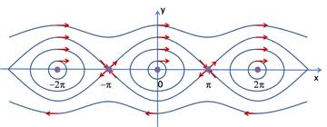
[from : http://mathematicalgarden.wordpress.com/2009/03/29/nonlinear-pendulum/]
Unfortunately this figure doesn't accurately reflect the different lengths of the velocity vectors. The equilibrium at
the origin is an elliptic point. The one at π is a hyperbolic point. The vector field vanishes at these points.

Tuesday, Nov. 15

- Lorentz contraction with spacetime diagrams: what is the line whose length is measured? It's the simultaneoity slice of the given
observer. So observers don't really disagree on the length of an object, they just differ on what length they are talking about.

- EM coupling: The action for the coupling of a charge needs no "relativistic correction", its already perfectly consistent with relativity,
whcih is no accident, since after all it was the properties of electromagnetism that led Einstein to discover relativity. The EM coupling action
is given by -q∫ A.ds, where A=(V, Ac) is the electromagnetic 4-vector potential, and ds=(dt, dx/c) is the spacetime translation and the dot is the
Minkowski dot product. [I didn't say this in class, but actually an even better way to say this is that the action is -q∫ A_mdx^m, where there is a
summation over the four values of m, dx^m are the components of ds, and A_m= (V, -A_ic), the index i being just the spatial part. I made the point
that just given the scalar potential term -q∫ V dt, relativity would tell you that dt can't stand alone, and that you had better replace V by a 4-vector.
(Alternatively you could invent a theory where V is a scalar and you replace dt by dtau.) Then the existence of magnetism, and Faraday's law,
would all just follow from relativity without any experiment!

- Gravitomagnetism: This is not something I addressed in class, but it seems worth mentioning for those who are interested.
In class it was explained how Now we can see that for weak gravitational fields there is a phenomenon that looks like a gravitational version of magnetism.
If we denote the Minkowski metric by g0_mn and the metric perturbation by h_mn, the proper time becomes dtau = √(g0_mn + h_mn)dx^m dxⁿ.
If we expand this in h and assume low velocities it becomes dtau = √(g0_mndx^m dxⁿ) + A_mdx^m + ..., where A₀= h₀₀/2, and A_i= h_0i.
So the 0i off-diagonal components of the metric perturbation act like magnetic vector potential. Why would we have such components? If the source mass
is moving relative to a given frame, then such components arise. For example, a spinning body like the earth produces a gravitomagnetic vector potential.

- Gravitational field equation for Newtonian and Einsteinian cases... Newtonian: gravitational force = mg, field equation is div g = -4πG rho_m.
The fact that div g = 0 in vacuum implies that tidal deformation is volume preserving to second order in time. Proof: consider a bunch of test particles
that start at rest. Their velocity after time t is v(x,t) = g(x,0) t + O(t^2), where I am labeling the particle by its position x at t=0. (The O(t^2) terms would
include the effect of the particle moving to another location where g has a different value, the fact that g itself might be changing in time, and the fact that
the particle in any case is accelerated.) It follows that div v = O(t^2). The significance of this is that a divergence-free velocity field generates a volume
preserving flow. One way to see this is to imagine a volume V in space. The divergence theorem tells us that ∫_V div v d(vol) = ∫_∂V v.da, where ∂V is the
surface bounding the volume V. If the divergence is zero, then the vector field has no net flux through the surface. But this flux describes the rate of change
of the volume with respect to time as the volume deforms under the flow. That is, dV/dt = ∫_V div v d(vol). For a small V we can approximate this integral by
(div v)V. Given that the divergence of the gravitationally induced velocity field is O(t^2) this means that our small volume of test particles satisfies
(dV/dt)/V = O(t^2). The volume as a function of time is thus V(t) = V(0) + O(t^3), there is no 2nd order change. If we are not in vacuum then instead
(dV/dt)/V = -4πG rho_m t, so V(t) = (1 - 2πG rho_m t^2) V(0) + O(t^3).

In general relativity the deformation of a volume of freely falling test particles is determined by the geodesic equation, which is determined by the line
element. The volume preserving at second order property carries over to general relativity for a bunch of test particles at rest in ANY local freely falling frame
in vacuum. In fact, this statement is equivalent to the vacuum Einstein equation. In the presence of matter, the mass density rho_m is replaced by the energy
density plus 3 times the pressure (if the pressure is isotropic). Here is an introductory article by Baez and Bunn explaining this viewpoint on Einstein's field equation.

Thursday, Nov. 10

- More on the rod hanging from a string (problem S7.3):
I wanted to sort of demonstrate, by comparing with a simple pendulum of length R/6,
that the frequency of the rapid mode in the case l >> R is indeed sqrt[g/(R/6)]. I didn't have a true simple pendulum but only
a sphere whose radius was perhaps half the length. But it seemed to match roughly. Hmm, let's figure out the period
of the sphere on a string. For any physical pendulum, we have a lagrangian L = 1/2 I thetadot^2 - Mgl(1-cos(theta)), where I is the
moment of inertia about the pivot, M is the total mass, and l is the distance from pivot to CM. The angular frequency w for small
oscillations is w = sqrt[Mgl/I]. The moment of inertia about the center of a uniform sphere of radius r is (2/5)Mr^2. Using the
parallel axis theorem we get I by adding to this Ml^2, so I=M(l^2 + (2/5)r^2). Thus the frequency is w = sqrt(g/l)/sqrt[1 + (2/5)(r/l)^2].
If r=l the correction is to multiply by 1/sqrt(1 + 2/5) ~ 1 - 1/5 = 4/5 = 0.8, i.e. about a 20% decrease in frequency. If r = l/2, which is
closer to the case we had, the correction is 4 times smaller, around 5%. So it was a reasonable comparison, given the experimental
uncertainty!

Then I went on to ask about the amplitude ratio in the modes when l = R, specifically the lower frequency mode, where it looks like
the pendulum is just swinging in a straight line. I spaced out and asked Justin to calculate the eigenvectors of the M matrix which
didn't make any sense, but Chris pointed out that I forgot about K! So we are looking for the w values and zero-eigenvectors of
w² M - K, which we can re-write as w² K(K^-1M - w^-2). Since w² K is invertible we can just peel it off, so we're looking for the
eigenvectors and eigenvalues of K^-1 M. (I write it this way, rather than inverting M, since K is easy to invert, being diagonal in this case.)
The eigenvalues will represent the reciprocal squared frequencies.

OK, so we have K = diag(1, 1/2), so K^-1 = diag(1, 2), and M = {{1,1/2},{1/2, 1/3}}, so K^-1M = {{1,1/2},{1, 2/3}}.
The eigenvector in the low frequency mode can be written as {1, 1.12} (I used the Mathematica "Eigensystem" to find this,
and evaluated the ratio of the resulting amplitudes.) So the lower angle amplitude is 12% more than the upper one. It was
not possible to really confirm this, even roughly, because I couldn't get the pendulum to swing just in this normal mode
without the other mode also excited. But now it occurs to me that I could perhaps have done that by driving the system at the
resonant frequency. Next class I'll try that!

- Compton scattering: I described the Feynman diagrams that contribute to Compton scattering at lowest order ("tree-level"),
just to fill in the picture. There are two diagrams. The incoming photon is destroyed, and a new photon is created.
A terrestrial application of Compton scattering is to radiation therapy: scattering gamma rays from electrons in the body
damages cells. The probability of an interaction is small and equal along the flight path of the photon. Intersecting beams of
photons are arranged to selectively target a tumor.

- Inverse Compton scattering: this is really just Compton scattering viewed in a frame in which the incoming electron
has a lot of energy that it transfers to a photon. It can "upscatter" photons into very high energies, and is relevant in high
energy astrophysics. Actually it also happens in terrestrial synchrotrons. See http://en.wikipedia.org/wiki/Compton_scattering
(At the GRenoble Anneau Accelerateur Laser they produce (polarized) gamma ray photons of energy 0.3 - 1.5 GeV by
colliding 6 GeV electrons with polarized UV laser light (3.53 eV photons).)

- a little more on the LHC and the Higgs particle: I put this info in last Tuesday's notes.

- General Relativity:

Background: Newtonian spacetime structure assumes 1) absolute time t, 2) spatial distance at constant time, 3) absolute rest or
family of inertial frames. Instead spacetime in special relativity is fully characterized by the Minkowski line element which
determines the proper time along any displacement. This encodes time, distance, and inertial structure all in one spacetime
geometry. (The inertial motions maximize the proper time.) Now where does gravity fit in to this?

Gravity and inertial force: Einstein focused on the extremely well known fact that the gravitational force is proportional to
the mass of the object it is acting on: F = mg, where g(x,t) is the gravitational field. This means that the effects of gravity can
be locally removed by using a "freely falling" reference frame with acceleration g relative to what a Newtonian would consider
an inertial frame. But Einstein proposed that we should think of it the other way around: the freely falling frame is the inertial one,
and then one interprets the gravitational force as an inertial force, due to working in a reference frame with acceleration -g.
So, for example, sitting in my chair, I am in a frame accelerating upwards relative to the local inertial frames.

Gravity as tidal field: While the local inertial frames can be identified with the freely falling frames, we must face the fact that
these frames are not the same everywhere. For example, at different points near the surface of the earth the free-fall frames
are falling inward radially, and the radial direction depends on where you are. Also the acceleration is greater closer to the earth than
farther. This is reflected in the simple fact that the derivatives of g are not zero, so that nearby freely falling particles have slightly
different accelerations. You could recognize this in a falling elevator: if release a spherical cluster of particles, as the cluster falls it
will deform to an ellipsoid, compressed in the transverse direction and stretched in the falling direction. The true essence of gravity
is this "tidal deformation". If it weren't for that, we could just cancel off gravity once and for all by changing the reference frame.

Spacetime curvature and the tidal field: Given that the inertial structure of spacetime is determined in special relativity by the line
element, it must be that a spatially varying inertial structure is described by a spatially vaying line element, that is, by a deformation
of the geometry of spacetime. In fact, the curvature of the spacetime geometry captures the notion of varying inertial structure.
As a concrete example, freely falling paths can start out parallel in spacetime, and be pulled togetther by the gravitational tidal
field. That parallel lines do not remain parallel is a sign of curvature. The motion of a test particle in such a spacetime is determined
by maximizing the proper time, using the line element of the curved geometry.

Spacetime geometry outside a spherical gravitating mass: Einstein's field equation for spacetime geometry has a unique spherically
symmetric, vacuum solution, up to one parameter corresponding to the mass M. That Schwarzschild metric can be expressed
using so-called Schwarzschild coordinates as

ds^2 = F(r) dt^2 - (1/F(r)) dr^2/c^2 - (r/c)^2 (dtheta^2 + sin^2theta dphi^2)

where F(r) = 1 - r_g/r, and r_g = 2GM/c^2 = 3km (M/M_sun) is the Schwarzschild radius. If M = 0 then F(r) = 1, and this is
just the flat spacetime, Minkowski line element in spherical coordinates. At r = r_g something goes wrong with the coordinates,
but the spacetime is fine there. This line element describes a black hole event horizon at r = r_g. For a star, the stellar surface lies
outside r_g, and the line element inside the star is not given by the Schwarzschild metric.

Cosmological line element: A simpler example of a curved spacetime is an expanding universe. If we average over the lumpiness
this can be described as a homogeneous, isotropic spacetime, with line element

ds^2 = dt^2 - a(t)^2(dx^2 + dy^2 +dz^2)/c^2

The function a(t) is called the scale factor, and it determines how much physical distance corresponds to a given coordinate displacement
dx, for example. Before the acceleration of the universe today was discovered, it was believed that a(t) was ~ t^2/3, so that the scale factor
was increasing with time with a rate ~ t^-1/3 that was decreasing in time. This would be "decelerated expansion". Now it appears that
infact the expansion rate is increasing. The simplest such increase, that would be caused by a cosmological constant, would be exponential,
a ~ e^Ht, in which case the rate would be exponentially increasing as well.

Newtonian limit of particle motion in the Schwarzschild field: The action for a particle of rest mass m is -mc^2 ∫ ds. For the Schwarschild
geometry this gives

S = -mc^2 ∫ ds = -mc^2 ∫ Sqrt[F dt^2 - (1/F) dr^2/c^2 - (r/c)^2 (dtheta^2 + sin^2theta dphi^2)]

                        = -mc^2 ∫ dt Sqrt[F - (1/F) (dr/dt)^2/c^2 - (r/c)^2 ((dtheta/dt)^2 + sin^2theta (dphi/dt)^2)]

If we restruct attention to values of r such that r_g/r << 1, and values of the velocity that a much less than the speed of light, we may expand the
square root and drop all but the leading order terms in r_g/r and v/c, in which case the action becomes

                       = -mc^2 ∫ dt [1 - GM/(c^2 r) - 1/2 v^2/c^2 + ...]

                       = = ∫ dt [-mc^2 + GMm/r + 1/2 mv^2 + ...].

This shows that the Lagrangian is a constant -mc^2 plus the Newtonian Lagrangian, plus corrections...

Tuesday, Nov. 8

- Went over the problem of the physical pendulum (linear rod) suspended from a string, and demonstrated the motion.

- 4-velocity: u = ds/dtau = (dt/dtau, d(x/c)/dtau) = (γ, γ/c dx/dt) = γ(1, v/c), where v is the usual 3-velocity v = dx/dt.
Note u^2 = u.u = (ds/dtau).(ds/dtau) = (ds.ds)/(dtau)^2 = 1. So the 4-velocity is a unit vector.

Consider two 4-velocities, u_1 and u_2. Their dot product is γ, the relative gamma factor between them. Why? Well let's evaluate it using
the components in the frame of u_1, so u_1 = (1,0,0,0) and u_2 = γ(1, v/c), so u_1.u_2 = γ.

- 4-momentum revisited: We can express a timelike 4-momentum in terms of the 4-velocity and the rest mass:

p = (mc^2) u

Squaring both sides (i.e. dotting with themselves) yields the mass shell condition, p^2 = m^2 c^4.

If we have two different timelike 4-momenta, p_1 and p_2, combining the previous results immediately yields

p_1.p_2 = γ m_1 m_2 c^4.

- Energy measured by an observer with 4-velocity u_obs is

E_obs = p.u_obs.

Why? Well in the rest frame of the observer u_obs = (1, 0, 0, 0) and p = (E_obs, p_obs c), from which it immediately follows.
So we can pick off the observed energy by dotting the 4-momentum with the observer's 4-velocity.

- Frequency measured by an observer: If k is the 4-wavevector, then in the frame of the observer we have k = (w_obs, k_obs c), so

w_obs = k.u_obs.

Doppler effect: If a source with 4-velocity u_s emits a photon with 4-wavevector k that is observed to travel at angle theta relative to the
motion of the the source by an observer with 4-velosity u_obs, what is w_obs? In the frame of the observer we have

u_obs = (1, 0, 0, 0)
u_s = γ(1, v, 0, 0)
k = (w_obs, w_obs khat) = w_obs(1, cos(theta), sin(theta), 0)

Thus w_s = k.u_s = w_obs γ(1 - v cos(theta)), which yields the relativistic Doppler formula,

w_obs = w_s/[γ(1 - v cos(theta))]

When theta = 0 this can be written as w_s Sqrt[(1+v/c)/(1-v/c)].
When theta = π this can be written as w_s Sqrt[(1-v/c)/(1+v/c)].
When theta = π/2 this is just w_s/γ. This is the transverse Doppler effect, which just arises from the time dilation between the frame of the
source and the frame of the observer.

Thursday, Nov. 3

"Look Ma, no Lorentz transformations" - Just as we rarely use rotations explicitly in nonrelativistic mechanics,
but instead make wise choices of coordinate systems and use rotational invariant quantities like magnitudes of vectors and
angles between vectors, we rarely need to use Lorentz transformations to relate the components of 4-vectors in different
reference frames. To simplify our lives, and focus on the most useful things, I will probably completely skip any discussion
of Lorentz transformations!

4-vectors: Form a four-component vector from a spatial vector vector and another component, the timelike component.
The prototype 4-vector is a spacetime displacement ds = (dt, dx/c). The invariant interval ds^2 = dt^2 - (dx.dx)/c^2 motivates
the definition of the Minkowsi inner ("dot") product:

ds^2 = ds.ds = (dt, dx). (dt, dx) = dt^2 - (dx.dx)/c^2

More generally, we define 4-vector by A = (A_t, A), where A is a spatial vector and A_t is a spatial scalar.
Given another 4-vector B = (B_t, B) we define the Minkowsi inner ("dot") product by

A.B = A_t B_t - A.B

For this formula to make sense the dimensions of A_t and A must be the same. (I'm relenting here and changing my
convention compared to what I said in class.)

NOTE: There are different conventions about 4-vectors. Taylor prefers to write the spatial vector first, and he defines the
iner product with the opposite sign. That is, Taylor would write A = (A, A_4), and for him

A.B = A.B - A_4 B_4    (15.50, Taylor)

energy-momentum 4-vector: Probably the most useful 4-vector is the energy-momentum,

p = (E, p c)

NOTE: Tayor defines it as p = (p, E/c)   (15.75, Taylor). The mass shell condition takes a neat form in terms of the
Minkowski inner product:

p^2 = p.p = (mc^2)^2

- The best way to handle the pesky factors of c is to ignore them! We can always choose our unit of length to be c times our
uit of time, and in such a system of units we have c = 1. If we want to express things in some other system of units we can use
dimensional analysis to insert the appropriate factors of c where they belong.

- photon + photon -> electron + positron makes the universe opaque to high energy photons, because of collisions with
cosmic microwave background (CMB) photons, or infrared (IR) background, depending on of far away the photon originates.
Energetics: the CMB has a temperature 2.7K. Note 1 eV/k = 11,600 K (where k = Boltzmann's constant), so 1 K ~ 0.1 meV,
so the typical CMB photon energy is ~ 0.3 meV. Because of this pair creation off the IR background we don't see photons above
about 50 TeV coming from farther than about 100 million light years away.

Center of momentum (CM) frame: Any collection of particles has some total 4-momentum P = p_1 + p_2 + .... There is always
a reference frame in which the total 3-momentum vanishes, called the center of momentum, or sometimes loosely, "center of mass"
frame. (The only exception is if all the particles are massless and have parallel momenta.) The invariant square of the total 4-momentum
is equal to the square of the CM frame energy:

P.P = (E_cm)^2.

Threshold energy to create particles: Suppose a moving particle with mass m_a collides with a particle of m_b at rest. Can these particles
disappear and create just one particle with a mass M? The total four momentum P = p_a + p_b is equal to the 4-momentum of the M particle, which
satisfies P.P = M^2. Thus

M^2 = P.P = (p_a + p_b).(p_a + p_b) = p_a.p_a + p_b.p_b + 2 p_a.p_b = m_a^2 + m_b^2 + 2 p_a.p_b

Let's suppose that m_b is at rest:

p_a = (E_a, p_a)
p_b = (m_b, 0)

so p_a.p_b = E_a m_b. Thus M^2 = m_a^2 + m_b^2 + 2 E_a m_b, or

E_a = (M^2 - m_a^2 - m_b^2)/2m_b

(multiply by c^2 to get the result in arbitrary units). Only if E_a has precisely this value can m_a and m_b annihilate to make M.
Moreover, since E_a cannot be less than m_a, M must be greater than or equal to m_a + m_b.

We can use this result to find the threshold energy to create a collection of particles at rest with masses {m_i}: at the threshold,
all the final particles will be at rest with respect to each other (minimum energy to create them), so to find this energy we can
just replace M in the previous calculation by the sum of the particle masses, M -> ∑ m_i.

Head-on vs. fixed target collsions: consider the case where the two colliding particles have mass m, so the threshold energy is

E^th = (M^2 - 2m^2)/2m.

Compare this to the threshold energy for a head-on collision: M/2 per particle. If M >> m the ratio of threshold energies for fixed target
vs. head-on is M/m.

Creating a Higgs particle at the LHC:
At the Large Hadron Collider (LHC) there are head-on proton-proton pp collisions, 3.5 TeV per proton currently. Assuming no physics
beyond the Standard Model (SM), the Higgs mass is currently constrained to lie in the range 115-140 GeV, or could possibly but uncomfortably
be > 450 GeV. (Note however that theorists consider it a good chance that ther is physics beyond the SM.) The dominant process
for making a Higgs particle in the SM is for a pair of gluons, one from each proton, to collide and make a Higgs particle via a top quark loop.
(Another contributor for example is when a quark and antiquark annihilate to make a W boson, which then emits a Higgs particle.)
If the gluons have equal energies that must be half the Higgs mass, i.e. ~ 70 GeV. The proton as a whole has 50 times more energy than this,
but the gluons inside the proton have only a fraction of the total energy. If the collision had one proton at rest, then the threshold energy to create
a Higgs particle with two protons would be ~ M_H^2/2m_p. The proton mass is 938 MeV ~ 1 GeV, so the threshold would be ~ (140)^2/2 ~ 10 TeV.
As just explained however, it's not the whole proton, but only constituent gluons that make the Higgs, and the gluons have only a small fraction of
the total proton energy. The rest of the energy goes into a pile of debris that is hard to makeout in general. I think they have to wait for the
rare cases in which the debris is clean enough to let them identify the Higgs by its characteristic decay patterns.

Compton scattering: I covered this as in section 15.6 of the textbook. First we relate a photon 4-momentum to the 4-wavevector p = hbar k = hbar(w, kc).
I used units with hbar = c =1. Calling the initial and final photon 4-momentum k0 and k, and the initial and final electron 4-momentum p0 and p, we have
energy-momentum conservation:

k0 + p0 = k + p,

and mass shell conditions k0^2 = k^2 = 0, and p0^2 = p^2 = m_e^2.
We can rearrarange 4-momentum conservation as k0 - k = p - p0. Taking the Minkowski dot product of each side with itself, and using the mass-shell conditions,
we find

- 2 k0.k = 2m_e^2 - 2p0.p   (*)

Now k0 = (w0, w0, 0, 0), k = (w, w costheta, wsintheta, 0), p0 = (m_e, 0, 0, 0) and p = (E, p), so

k0.k = w0 w (1 - costheta), and p0.p = m_e E = m_e(m_e + w_0 - w), where the last step follows from energy conservation. Eqn (*) thus yields

w0 w (1 - costheta) = m_e(w_0 - w), or

1/w - 1/w0 = (1 - costheta)/m_e

Using w = 2π/lambda and restoring the factors of hbar and c this becomes

lambda - lambda0 = (h/(m_e c))(1 - costheta)

The largest energy transfer happens when the photon scatters backward. Zero transfer happens in forward scattering.
The differential cross section depends on the photon polarizations. Summing over final polarizations and averaging over initial
ones yields the formula shown here: http://en.wikipedia.org/wiki/Klein–Nishina_formula.

Tuesday, Nov. 1

- relativistic energy and momentum

As explained Oct. 20, the relativistic action for a particle of mass m is S = - mc^2 ∫ dtau = - mc^2 ∫ dt √1-(dx/dt)^2/c^2 = ∫ L dt,
where the Lagrangian is defined by

L = - mc^2 √1-(dx/dt)^2/c^2.

The momentum conjugate to the veocity dx/dt is p_x = ∂L/∂(dx/dt) = γ m dx/dt, where the "gamma factor" is defined by

γ = 1/√(1 - (v/c)^2).

Thus the relativistic definition of 3-momentum is

p = γ mv.

The energy can be computed as the value of the Hamiltonian, H = v.(∂L/∂v) - L = γ mv^2 + mc^2/γ = γ mc^2(v^2/c^2 + 1/γ^2) = γ mc^2,

E = γ mc^2.

While E depends of course on the reference system (the "inertial observer"), the mass m has an invariant meaning, namely, mc^2 is the
"rest energy", i.e. the energy in the rest frame of the particle.

The energy and momentum are related in a simple way:

E^2 - (|p|c)^2 = m^2 c^4 ("mass shell formula")

Note that while the values of E and p depend on the reference system, the mass m can always be computed from them using the mass shell
formula. This is closely analogous to the situation with the proper time: while dt and dx depend on the reference frame, the squared proper time
dtau^2 = dt^2 - (dx.dx)/c^2 has an invariant meaning and can be computed from dt and dx in any reference frame.

We can take a limit m to zero and still have nonzero energy and momentum if the speed v approaches c. Massless particles thus satisfy

E = |p|c.

We can express velocity directly in terms of momentum and energy:

v = p/(E/c^2).

- non-relativistic limit: expand

γ = 1 + 1/2 (v/c)^2 + 3/8 (v/c)^4 + 5/16 (v/c)^6 + ...

so the expansion of the energy is

E = mc^2 + 1/2 mv^2 + 3/8 m v^4/c^2 + ...

At v = 0 there is only the rest energy mc^2. The next term is the nonrelativistic kinetic energy. The remaining terms are relativistic
corrections to the kinetic energy. The relativistic kinetic energy is defined as everything but the rest energy, T = E - mc^2 = (γ - 1)mc^2.

- example 5.8 from textbook

- example (problem 15.60): a particle of mass m_a decays at rest to a pair of particles of mass m_b. What is the speed of the final particles?
Apply energy and momentum conservation, and the mass shell condition. The total momentum is initially zero so the final momenta are
equal and opposite. Then the mass shell condition implies the final energies are equal, and energy conservation implies the energy of one
of the final particles is half the initial rest energy, E = 1/2 m_a c^2. We can get the velocity by setting this equal to γ m_b c^2, i.e.
γ = (m_a/2m_b). Solving for v yields v/c = √1 - ((2m_b/m_a)^2. Alternatively, the mass shell condition then gives us the magnitude of
the momentum, p = √(E/c)^2 - m^2 c^2, so the speed is given by v/c = p/(E/c) = √1 - (mc^2/E)^2 = √1 - ((2m_b/m_a)^2.

Thursday, Oct. 27 - Exam 1

Tuesday, Oct. 25 - review for Exam1

Thursday, Oct. 20

- proper time - in SR, time is "arclength" along a timelike curve. That is, the time between two events in itself is not
defined. Time is a proprty of a path in spacetime. This explains the twin effect: the relative aging of the twins can differ
if they travel different paths. I emphasized the analogy with path length in Euclidean geometry.

- spacetime interval - The interval is what determines times and lengths and the lightcone, as well as the inertial motions.
Logically, one should just postulate it, and derive consequences. But we can also motivate it and its properties, by just appealing
to the postulates of relativity and applying them to what are assumed to be inertial motions, i.e. straight timelike paths in spacetime.
We also call these "observers". Consider two obervers O1 and O2 who pass through the same event E and are moving relative
to either other. Let the zero of time correspond to the event E for both O1 and O2. At time t1 from E along his worldline, O1 sends
a light pulse to O2. The pulse is received at event F at time t0 on O2's worldline, and the reflected pulse arrives back at O1 at t2.
Then t0/t1=t2/t0, because each pair of times is defined by a similar experiment: same relative motion, events conected by a light pulse.
Thus the "radar relation" between the time measurements of O1 and O2 is

t0^2 = t1 t2. (*)

O1 would define the "time separation" Dt of the events E and F to be the time halfway in between t1 and t2, i.e. Dt = (t1+t2)/2. Similarly,
O1 would define the "distance" Dx from himself to F by the light travel time (t2-t1)/2 times the speed of light c, i.e. Dx = c(t2-t1)/2.
We can invert these definitions to find t1 = Dt - Dx/c and t2 = Dt + Dx/c, so (*) implies

t0^2 = Dt^2 - (Dx/c)^2. (**)

This shows that the proper time t0 of O2 along the straight path from E to F can be expressed in terms of the Dt and Dx coordinate increments
conventionally defind by O1 by a kind of Pythagorean theorem. Another observer O3 would define different coordinate increments Dt' and Dx',
but would get the same combination for the rhs of (**), i.e. Dt'^2 - (Dx'/c)^2 = Dt^2 - (Dx/c)^2, because they are both is equal to the square of
O2's proper time, t0^2. This invariant quantity is called the "(squared) spacetime interval".

Sometimes the spacetime interval is just called the "interval", and sometimes the "invariant interval". Sometimes it is defined with the opposite sign,
and sometimes multiplied by c^2 (hence given in length rather than time units), or both. For timelike displacements the squared interval is positive
as I've defined it, while is negative for spacelike displacements and zero for lightlike ones.

O1 would define the velocity of O2 as v = Dx/Dt. In terms of v, the square root of (**) becomes

t0 = Dt √1- (v/c)^2,

which is the famous relativistic time dilation formula: the proper time t0 measured by O2 along his own path is shorter than the time Dt assigned
to that path by O2.

- The interval is zero on a piecewise lightlike path that connects two events. The path of longest time is the inertial motion (straight line).

- The proper time along an arbitrary path is the integral of the proper time increment dtau:

proper time = ∫ dtau = ∫ dt √dt^2-(dx/c)^2 = ∫ dt √1-(dx/dt)^2/c^2.

We imposed the condition that the variation of the propert time is zero when the path is varied. This should be satisfied at the inertial path,
since that maximizes the proper time. Using the Euler-Lagrange equation, we showed that indeed a constant velocity path satisfies this maximum time condition.

- We took a nonrelativistic limit to understand the relation between the proper time and the non-relativistic action. Expanding in powers of v/c, the proper time
along a path is

proper time = ∫ dt √1-v^2/c^2 = ∫ dt (1- 1/2 v^2/c^2 - 1/8 v^4/c^4 + ...).

If this is multiplied by -mc^2 we get (-mc^2) ∫ dtau = ∫ (-mc^2 + 1/2 mv^2 + 1/8 m v^4/c^2 + ...). So we see that the -mc^2 times the proper time gives
a relativistic generalization of the action. The rest energy mc^2 acts like a constant potential energy. The second term of the integrand is the nonrelativistic
kinetic energy.

Tuesday, Oct. 18

- Reviewed coupled oscillators and how to solve for the normal modes and frequencies using the matrix method.

- Discussed the oscillating systems that appear in hw7:
(CO₂ vibrations, masses suspended by springs, physical pendulum, physical penulum hanging from a string)

- physical pendulum: Lagrangian, in terms of the moment of inertia about the rotation axis.
D2-13 RACING PENDULA example.

- parallel axis theorem for moment of inertia. I showed that this is directly related to the decomposition of kinetic
energy into T = T_cm + T_rel. That is, For a rigid body rotating about a fixed axis, T = 1/2 I_axis thetadot^2,
while T_rel = 1/2 I_cm thetadot^2 and T_cm = 1/2 M R_cm^2 thetadot^2. Here I_axis and I_cm are the moments
of inertia about the axis of rotation and about a parallel axis through the center of mass. The equality of these two
representations of the kinetic energy implies I_axis = I_cm + M R_cm^2, the parallel axis theorem.

- special relativity: To write the Lagrangian or Newton's second law we use certain structures that are assumed
present in spacetime in order to define velocity, speed, and the action:
1) absolute time function t, 2) metric of spatial distance at one time, 3) family of intertial frames.
(Newton replaced 3) by an absolute standard of rest, but Newtonian physics only depends on the family
of inertial frames, not on which one of those frames is used as the standard of rest.) In special relativity, all of these
structures are unified into one, the spacetime interval. Before we get to the quantitative aspects of relativity, let's
discuss the qualitative aspects...

The key fact giving rise to special relativity theory, historically, is that the speed of light as described by electrodynamics,
and measured by experiments, does not depend on the speed of the source, nor on the speed of the observer. [More
generally, the symmetry group of Maxwell's equations is not the Galilean group, but the Lorentz group.] This means
that the paths followed by light rays in spacetime trace out an absolute structure that is a property of spacetime.
This can be visualized as a lightcone at each spacetime event. Instead of an absolute time slicing of spacetime like
in Newtonian physics, we have an absolute family of light cones. At an event p, the inside of one half of the lightcone
is the future, the inside of the other half is the past, and the rest is the elsewhere. Points in the future or past of p are
timelike related to p, points in the elsewhere are spacelike related to p, and points on the cone are lightlike related.
The point p can only be influenced by events inside on on its past lightcone, and can only influence events inside
or on its future lightcone. So the lightcones define the causal structure of spacetime. [In Newtonian physics, the causal
structure is defined by the absolute time function.]

In Newtonian spacetime events at the same absolute time are simultaneous. In relativity, there is no absolute meaning
of simultaneity. A given observer can use radar to to define a notion of simultaneity, but that notion will depend on the
observer. Spacelike related points are always "simultaneous" as defined by some observers and not by others.
Timelike or lightlike related points are never simultaneous as defined by any observer.

Diagrams illustrating the relativity of simultaneity, and contrasting Newtonian and relativistic spacetimes.

Thursday, Oct. 13

Prof. Chacko covered the material in sections 11.1,2,4 of the textbook.

Tuesday, Oct. 11

- Perturbations of Mercury's orbit: solar oblateness, other planets. Apparently you can treat the planet as if it were a ring
of matter, to simplify the problem. I explained why the potential has a maximum in the center of the ring so it's like a
-ar^2 potential to the first approximation. (For a nice but somewhat complicated explanation of this method see
http://www.mathpages.com/home/kmath280/kmath280.htm. I don't know exactly how to fully justify the ring approximation,
but it seems plausible.)

- Le Verrier computed the planetary contributions (I think by this ring method) and they add to around 527 arcseconds per century.
The GR correction is 43 arcseconds. Le Verrier suggested the extra 43 arseconds might be due to a planet Vulcan in orbit between
Mercury and the sun (in class I incorrectly said it might be like an earth orbit, behind the sun).

- Dark matter: explained briefly a bunch of evidence for dark matter, and its properties. One example was the famous
bullet cluster of galaxies. (See also the Wikipedia article.)

- Tides: Finished discussing tides. Explained that the surface of the ocean should be an equipotential surface of the combined
gravitational and tidal potentials, and this this can be used to determine the height of ideal tides on an ocean covered earth (see
textbook for details).

- Rotating frame of reference: showed Rotating reference frame: movie, then wrote down the Lagrangian for free particle
motion in a plane as described in a uniformly rotating frame of reference. phi_in = phi_rot + Omega t, where Omega is the angular
velocity, so phido_in = phidot_rot + Omega. Insert this into the kinetic energy to find the Lagrangian

L = 1/2 m rdot2 + m r^2 Omega phidot + 1/2 m r^2 Omega^2

The second term is the velocity dependent Coriolis potential, and the third term is minus the centrifugal potential.
The Coriois potential is exactly what you'd get for a uniform magnetic field perpendicular to the plane, and the centrifugal
potential is an unpside down oscillator potential.

Rotating water tank & parabolic surface: movie shows that the surface of water in a rotating tank assumes a parabolic form.
We can understand this as for the surface of the oceean tides: the surface must be an equipotential surface of the combined
gravitational and centrifugal potentials. (The only other force, water pressure, is normal to the surface.) Thus
mgh - 1/2 mr^2 Omega^2 = const, i.e. h = (Omega^2/2g)r^2.

- 3d Coriolis and centrifugal forces: explained the nature of eqn (9.34) but did not derive it. (I suggest you go through the derivation
in the book, and ask me if you have questions.)

- Lagrange points: explained why these stationary points exist for test masses, and discussed their stability properties. L4 and L5 are
actually the top of the hill of the velocity independent part of the (combined gravitational and centrifugal) potential, but the Coriolis
force stabilizes motion around them, provided the ratio of the mass of the sun to the mass of the earth (or other planet) is greater than
about 25, which it certainly is. The location of L1,2,3 are easily found using standard force balance in Newtonian mechanics; I haven't
tried to fnd the location of L4 and L5 this way but I suppose it's also pretty straightforward. The analysis of the stability, being concerned
with time-dependent motion, is (or so I hear) easier to carry out in the rotating frame. For a detailed discussion of all this there are some
nice notes by Neil Cornish.

Thursday, Oct. 6

- In general relativity there is, in addition to the Newtonian terms -a/r + b/r^2, a term -d/r^3 in the effective radial potential
for orbits arounda central mass. Here a = GMm, b = l^2/(2m), and d = b r_g, where r_g = 2GM/c^2 is the "gravitational radius"
or "Schwarzschild radius" (for M = M_sun the gravitational radius is 3 km), and c is the speed of light. The ratio of the relativistic
term to the centrifugal barrier is r_g/r, which is tiny for a normal star, but can approach unity for a neutron star or black hole.
In general relativity this potential governs the radial velocity dr/ds, where ds is the proper time of the planet, and r is the
of the circumferential radius C/2π.

For Mercury's orbit around the sun the -d/r^3 term produces a very small contribution to the perihelion precession, the
famous 43 seconds of arc per centrury. (1 second = 1/3600 degree.)

For orbits close to a black hole the -d/r^3 term dominates, so there are no stable circular orbits very close to the black hole.
The innermost stable (actually marginally stable) circular orbit is called the "ISCO". The accretion disk around a black hole
has an inner edge at the ISCO. For spinning black holes the ISCO is closer to the black hole the higher the spin is. For a
maximally spinning black hole the ISCO coincides with the event horizon. This dependence of the ISCO on the spin
of the black hole is used to observe the spin: a spectral line emitted by iron atoms in the accretion disk is observed. The
the line suffers Doppler redhift, as well as gravitational redshift. The maximum redshift is determined by the mass of the
black hole and how close to the horizon the radiation is emitted. It also depends on the inclination of the disk to the line
of sight, whcih cannot be directly observed, but can be extracted from the maximum blueshifted part of the line, which is
Doppler shifted by motion towards the observer, and is largely independent of the black hole spin.

- Showed that Kepler's 2nd law (equal areas swept out in equal times) is equivalent to angular momentum conservation.

- noninertial frames: Explained as in the textbook. If the acceleration of the frame is A, Newton's law for a mass m in that
frame includes an inertial force -mA. This is also sometimes called a ficticious force, or a pseudo-force.

- How to spot an inertial force: it is proportional to the mass of the particle. (Note there is another kind of force that has this
propertty: gravity! Einstein took this to mean that gravity is actually not a real force but an inertial force...more on this later.)

- vertically accelerating elevator example.

- horizontally accelerating car example as in book.

- Tides: The change in strength and direction of the moons force over the surface of the earth produces the tides.
The high tides due to the moon are around midnight and noon at a new moon or full moon, and around sunrise and
sunset for a 1/4 or 3/4 moon. The sun contributes about 1/2 as much as the moon to the tides on earth. When the sun
and moon are aligned, at new moon or full moon, the tides are larger, and are called spring tides. When the moon is
at 1/4 or 3/4 phase, the tides are smaller, and are called neap tides. The tidal bulge actually is actually afew degrees
ahead of the moon in the direction of the earth's rotation. I think this is due to the lag of the response of the ocean to
the changing moon force in the earth centered reference frame. Details of tides depend of course on the local flow
features induced by the presence of land forms.

- Computation of tidal force, as in textbook. The tidal force is the difference between the lunar force at a point on the surface
of the earth and the lunar force at the center. Ended writing the tidal potential from which the tidal force can be computed
by taking minus the gradient.

Tuesday, Oct. 4

- discussed some of the hw problems a bit

- reviewed the reduction of the 2-body problem to one body in a 1d effective potential

- derived the elliptical orbit shape

- discussed Kepler's 3rd law period^2 = [(4π)^2/GM](semimajor axis)^2. I expressed my puzzlement that this relation is independent of
the ellipticity of the orbit. There has to be a deep reason for this.

- Closed orbits: They are closed in general only for 1/r^2 force and harmonic oscillator. Perturbations from oblateness of the sun, or from Jupiter,
or from the general relativity correction, can make the orbits slightly not closed, so they precess.

We discussed another way to show that the orbits are closed, in the approximation of small ellipticity. This method will allow the small
precession rate to be computed when the potential is perturbed. The method is to compare the frequency of radial oscillation with the frequency
of angular oscillation. For an effective potential of the form U_eff = a/r^2 - b/r, there is a circular orbit at U_eff' = 0, i.e. r = r_0 = 2a/b.
The radial oscillation frequency is omega_r = sqrt[U_eff''(r_0)/µ]. Now U_eff'' = 6a/r^4 -2b/r^3 = (2/r^4)(3a - br),
so U_eff''(r_0) = 2a/r_0^4, and omega_r = sqrt[2a/(µr_0^4)]. On the other hand, the angular frequency can be expressed in terms of the angular
momentum as omega_phi = phidot = p_phi/mr^2. If the 1/r^2 term comes completely from the centrifugal barrier, then a = p_phi^2/(2µ), so the
two frequencies agree. Otherwise they differ.

- L_tot = L_cm + L_rel, where L is the angular momentum. Applied this to see that in terms of the reduced mass µ and the separation vector r,
the angular momentum relative to the center of mass is L = µ r x rdot, whose magnitude is µ r^2 phidot, so this is in fact the same as the conserved
quantity p_phi = ∂L/∂phidot.

Thursday, Sept. 29

- comments about soap film problem, the unstable solution, and the critial separation

- comments about the catenary problem

- overview of 2 body problem:
= reduction to free particle motion of center of mass, and effective one body problem of motion relative to the center of mass
= for central forces, angular momentum conservation solves the angular problem, reducing to an effective 1d problem in an effective potential

- dedfinition and properties of the center or mass and position and velocity relative to the center of mass

- T = T_cm + T_rel

- 2 body problem, Lagrangian and effective potential for the relative motion

- qualititative properties of orbits

- equation for the shape of the orbit in terms of u(phi), where u = 1/r, and r is the separation of the bodies, and phi is the angle of their separation vector.

We ended at equation (8.45). Several things were derived and/or explained somewhat differently from inthe book.

Tuesday, Sept. 27

- ambiguity of Lagrangian under addition of (d/dt)f(q,t): clarified why f must not depend on derivatives of q.
(See last Thursday's notes for more details).

- gauge invariance of electromagnetic part of Lagrangian: showed that both the -V and v.A terms are needed together,
and with exactly the relative coefficient -V + v.A, in order for a gauge transformation to just produce a total time derivative.
(See last Thursday's notes for more details).

- Lagrange equations for charged particle in electromagnetic (em) field: showed how the em term q(-V + v.A) produces
the Lorentz force law. I did this using an index notation, with Cartesian coordinates, because it's good to learn about
index notation. (I neglected to emphasize at the beginning that I was using Cartesian coordinates. We can easily
generalize the method to arbitrary coordinates - we'll to that later.)

- Lagrange multipliers:
This is more complicated, so I've also prepared a latex version of Lagrange multipliers and constraints you might prefer.

Start with multivariable calculus: suppose f(x,y,z) is constant on the z = 0 surface. Then although
we can't say that grad f = 0 when z = 0, we can say grad f = lambda zhat when z=0. OK, I have an html problem here with notation.
Let me use df for the gradient of f, and w for the Lagrange multiplier, so the last equation would be written df = w zhat.

Now let's generalize this example to consider a function that is constant on a surface defined by a constraint equation
C(x,y,z) = 0. Then df must be parallel to dC when C = 0. Put differently,

df = w dC when C = 0, for some function w.

In the example C = z, so dC = zhat, and this agrees with what we just said above.
Another way to see that this is the right condition is to take the dot product with an arbitrary vector v, which gives
v.df = w v.dC. If v is tangent to the constraint surface then v.dC = 0, so in that case the equation implies v.df = 0, i.e.
the rate of change of f along the directions that lie in the surface is zero. For v that is not tangent to the surface, f can change.

Now what if there are two constraints? For example C₁ = z and C₂ = x² + y² + z² - R². So C₁ = C₂ = 0 implies the point
is both on the z = 0 plane and on the sphere of radius R. That is, it lies on the circle of radius R in the xy plane, centered on the
origin. The gradient of a function that is constant on this circle must satisfy df = w₁ dC₁ + w₂ dC₂ when C₁ = C₂ = 0. This is
equivalent to saying that the derivative of f in any direction tangent to both constraint surfaces is zero.

One more formal point before applying this to Lagrangians: Instead of writing df = w dC we can equally well write
df = d(wC), because d(wC)= w dC + C dw, and when C = 0 the second term vanishes. So the condition on f can also be
written as d(f - wC)=0 when C = 0. Since w is undetermined at this stage anyway, we can also flip the sign and write this
condition as

d(f + wC)=0 when C = 0.

If we have two constraints, the condition can be written as d(f + w₁C₁ + w₂C₂) = 0 when C₁ = C₂ = 0.
The generalization to any number of constraints is obvious.

- Lagrange multipliers and mechanics:

Let's illustrate how this applies to constrained mechanics with an example. Cconsider the
simple pendulum of length R. We've seen we can just impose the constraint r = R from the beginning, using the angle theta as our
sole generalized coordinate. This is equivalent to just demanding that the action be stationary with respect to variations of the path
(r(t), theta(t)) that respect, for each time t, the constraint C(t) = r(t) - R = 0.

This constrained variational principle on the action functional S[r(t),theta(t)] is just like what was discussed above for functions.
Instead of one or two constraints however we have an infinite number of constraints C(t) = 0, one for each t. If we add them all to S,
multiplied by a Lagrange multiplier function w(t) and integrating over t, we arrive at an equivalent, but unconstrained variational
principle: the variation of S + ∫ w(t)C(t) dt should be zero for any variation, when C(t) = 0 holds. Or, in terms of the Lagrangian, the
variation of

∫ (L + wC) dt

must vanish (the t-dependence of w and C is not explicitly indicated but it's there).
So in the end it's quite simple: we just add to the Lagrangian an arbitrary multiple of the constraint(s).

For the pendulum, the theta equation is unchanged, but now that r is not fixed a priori we get an r equation
of motion. The action is the integral of L + wC = 1/2 m rdot^2 + 1/2 m r^2 thetadot^2 + mgr cos(theta) + w(r - R), so the r equation is

m rddot = mr thetadot^2 + mg cos(theta) + w,

where the w term comes from ∂(wC)/∂r when C = 0. Recall that this is supposed to hold only when the constraint C = r - R = 0 holds,
so it is really the condition

0 = mR thetadot^2 + mg cos(theta) + w.

Since w is so far an arbitrary function this doesn't impose any condition on anything else, of course. In fact, we can solve this equation for w,

w = - mR thetadot^2 - mg cos(theta).

- Forces of constraint:
What is the meaning of w? It's whatever it must be for the r equation of motion to be satisfied when r is fixed at r = R. So w must be closely
related to the force of tension of the string. In fact, in this case, it is exactly the tension force, as we can see with a Newtonian calculation:
the force in the radial direction is the radial component of the gravitational force minus the tension: mg cos(theta) - T, where T is the magnitude
of the tension force. The radial acceleration is the centripetal acceleration - R thetadot^2. The radial component of F = ma then yields
T = mg cos(theta) + mR thetadot^2. Hence w = -T. The minus sign is because this force is in the negative rhat direction.

What is the general relation between the Lagrange multiplier w(t) and the force of constraint? The answer is simple: whatever the wC term
produces in the equation of motion, that is the generalized force for the corresponding generalized coordinate. That is, w ∂C/∂q is the generalized
force. In the pendulum example, C = r - R, and the coordinate is r, so dC/dr = 1, and w is just the constraint force in the r direction. If the
constrained coordinate q had been an angle, w ∂C/∂q would be the torque of constraint. If q is some more unusual generalized coordinate,
then we'd just have some unusual generalized force of constraint. [If C depends on time derivatives, then in general things are trickier
(non-holonomic constraints), but if the constraint can be used to eliminate a coordinate it is more or less the same.]

Thursday, Sept. 22

Free particle at rest: v = 0 path has the minimum action, S = 0.

Freely falling particle in uniform gravitational field: minimum action negative, from up and down motion.
If particle goes up a height h, both v and U scale proportional to h, but T scales as h^2. So for small enough
h, the Lagrangian T - U will be negative. The h that gives minimum for constant velocity up and down happens
to be the same as the h that gives the height of the classical path. (Can you find an argument showing that this
must be the case?)

If you bring in circular orbits then, for a sufficiently long time interval, there is a second path, the circular orbit.
The action on that path is a saddle point of the action, not the minimum.

Ambiguity of the Lagrangian: You can add a total time derivative without changing the equations of motion,
because the action for L + df/dt is the action for L plus [f(t_2) - f(t_1)]. With fixed endpoints, these actions differ
by a constant (asuuming f = f(q,t) depends on q and t but not on time derivatives of q), so they have the same
stationary points. A nice example is in the homework, of the pendulum in an accelerating elevator.

Change of inertial frame (Galilean transformation): What is the change of the action when you change
inertial reference frames? The definition of kinetic energy changes: the velocity wrt the new frame is v' = v - v_0,
where v_0 is the velocity of the new frame wrt the old one. The kinetic energy in the new frame is therefore

1/2 mv'² = 1/2 m v² - mv_0 v + 1/2 m v_0².

The difference of the two definitions of kinetic energy is a total time derivative: T' = T + df/dt, with
f = (-mv_0 x(t) + 1/2 mv_0^2 t). The definition of potential energy doesn't change since it is just a function U(x,t)
of position in space and time, which makes no reference to a particular frame. (Of course the formula for it
would look different when written using the new coordinate.) So the Lagrangian changes by a total time
derivative, so the action changes by a constant, for fixed endpoints.

Using this we can argue that the free particle motion at constant velocity minimizes the action: go into the
reference frame where the velocity is zero, where clearly the action is minimized.

Electromagnetic force: Lorentz force law: F = q(E + v x B).

For electrostatic fields we have E = - grad V, and the electrostatic potential energy of a charge is qV,
which can be used in the Lagrangian to get the equation of motion. But if the electric field has a part
that is induced by a changing magnetic field, then E is not the gradient of a scalar. Moreover, if there
is even a static magnetic field, how do we handle that?

I explained how Faraday's law, curl E = - ∂_tB, and the absence of magnetic poles, div B = 0, imply that
there exists a scalar potential V and vector potential A such that B = curl A and E = - grad V - ∂_tA.
The potentials are not unique: one can make the gauge transformation to new potentials

A' = A + grad f, V' = V - ∂_tf

which yield exactly the same B and E. This is called gauge invariance of the fields.

Now, what about the Lagrangian? There are many conditions to be satisfied.
The electromagnetic term should be

1) a scalar - the action is a scalar
2) linear in the potentials - since the Lorentz force is linear in the fields
3) gauge invariant - since the equation of motion involves only the fields, not the potentials

We can guess there is a term like in the electrostatic case, -qV. This is a scalar and linear in V.
It is not gauge invariant, however, since V changes by ∂_tf. If this were a total time derivative with respect to t it
would not change the equations of motion, but it is only the partial derivative. So this can't be the whole story,
because the Lagrangian is not gauge invariant, even up to a total time derivative. But we haven't finished.
There is also the vector potential. It's a vector, so to make a scalar that is linear in the vector potential we need
to form its dot product with another vector. To maintain linearity, that other vector should be independent of the
potentials. There is only one such vector available: the particle velocity!
So we guess that the term we need is proportional to v.A.

Now what about the third criterion, gauge invariance? Under a gauge transformation, v.A changes by
v.grad f. Since v = dx/dt, this looks like a time derivative, v.grad f = df/dt, but that's not quite right!
The t dependence of f(x(t),t) comes in both via x(t) and through explicit time dependence, and v.grad f
picks up only the former. It doesn't include the explicit time dependence. But remember that the gauge change of the
scalar potential term involves only the explicit time dependence. So, taken together, the scalar and vector
terms are gauge invariant if we add them in the combination v.A - V. Under a gauge transformation this combination
changes by the total time derivative df/dt! So to satisfy the three conditions above, we seem to have
no choice but to define the electromagnetic part of the Lagrangian as L_em = q(v.A -V).

Tuesday, Sept. 20

Spherical pendulum again: how to set up the problem if there is motion in both the theta and phi directions.
Write out both equations of motion. The phi equation will be the the angular momentum conservation law,
and enables one to solve for phidot in terms of the conjugate momentum p_phi and theta. Then this can be used
to eliminate phidot from the theta equation, reducing the theta motion to a one dimensional problem with
an effectve potential U_eff(theta). Important note: you cannot substitute for phidot in terms of p_phi in the
Lagrangian before finding the theta equation. This would introduce theta dependence that is different from
what was in the Lagrangian. It's incorrect, because this extra theta dependence comes from the relation between
phidot and p_phi, treating the arbitrary conserved p_phi as a constant.

- small oscillations of the spherical pendulum: We showed before that for any fixed theta_0 there is a circular
motion, with some associated angular momentum. Now you can perturb that motion to introduce an oscillation,
whose frequency will be determined by w^2 = (U_eff)''(theta_0).

Spinning hoop: made several points about this.

1) The mass drops out of the equations of motion. It affects the forces of constraint, but as the Lagrangian is proportional
to m, not the equations of motion. This derives from the fact that both the inertia and the force of gravity are proportional
to m. This is of course a special property of gravity.

2) We can choose units with m = g = R = 1. This simplifies the equations, but you loose the ability to check your
algebra with dimensional analysis. You put the m, g, R back in at the end using dimensional analysis.

3) Went over the solution of the problem of small oscillations about the equilibrium points in detail. Showed how the
evaluation of (U_eff)''(theta_0) is simplified by writing (U_eff)'(theta) as a product of factors, one of which vanishes
at each equilibrium point. Only the derivative of the latter factor survives when evaluating (U_eff)''(theta_0).

Conservation of energy: momentum and angular momentum conservation derive from space translation and
rotation symmetry respectively. Energy conservation arises from time translation symmetry. We derived the conserved
quantitity that arises from time translation symmetry of the Lagrangian. If there is no explicit t dependence in L, then
the "Hamiltonian", H = p_i qdot^i - L, is conserved. Here the index i appears twice, once on p_i and once on qdot^i.
We use the Einstein summation convention according to which reapeated indices appearing in the same term (i.e. on
multiplied objects) are summed over all their values. What is the meaning of H? For a Lagrangian of the form
L = 1/2 A_ij(q) qdot^i qdot^j - U(q) we find H = 1/2 A_ij(q) qdot^i qdot^j + U(q). So if the kinetic energy is
T = 1/2 A_ij(q) qdot^i qdot^j, then H = T + U is the total mechanical energy.

Index gymnastics: In deriving the form of H in the previous paragraph, we went through some index gymnastics.
I will write some latex notes about this.

We considered a relatively simple example where H is not the total mechanical energy: the bead sliding on a
hoop driven by an external torque to rotate at constant angular frequency omega. The Lagrangian is
L = 1/2 m R^2 thetadot^2 + 1/2 m R^2 sin^2(theta) omega^2 - mgR(1-cos(theta)). The second term is the azimuthal
part of the kinetic energy, but it contains no time derivatives of the generalized coordinate theta, so shows up as a
contribution to the effectve potential U_eff(theta). This means that H is not the total mechanical energy, but rather
the total mechanical energy minus twice the azimuthal kinetic energy. It makes sense that mechanical energy is
not conserved, since the driver of the rotation of the hoop puts energy into the particle motion. And the orientation of the
constraint forces is imposed by external time dependence, so the system really has time dependence, even though
the Lagrangian for the generalized coordinate does not. Also, angular momentum is not conserved, since the hoop
at each instant is an external constraint that violates rotational invariance. So what is H, this conserved quantity.
Is there a symmetry that it corresponds to??

Thursday, Sept. 15

- What is action? For a free particle motion the action is S =∫ 1/2 mv² dt, which is the average kinetic energy
times the total time interval. On the classical path (solution to the equation of motion) v = v0 = const. We
can easily show this is the minimum for all paths. In the presence of a potential, the action is still a minimum
on the classical path, provided the two times are close enough. For a harmonic oscillator, "short enough" means
less than half the period.

- Can change variables freely in describing the configuration of the system. Example: change from x1 and x2 to
x_cm and x_rel. (See this week's homework.)

- Constraints: Example of pendulum: can move in theta and phi, but not r. The r degree of freedom is constrained.
We can just leave it out of the Lagrangian, as the contraint ensures that the eqn of motion for it is satisfied.
Lagrangian for this pendulum in terms of theta and phi. Considered two cases: planar motion (phi = const) and
circular motion (theta = const). phi doesn't appear in the Lagrangian, it is an "ignorable coordinate", i.e.
phi translation is a symmetry. Correspondingly, ∂L/∂phidot, the "generalized momentum conjugate to phi", is conserved.
This is nothing but the angular momentum about the vertical axis. Showed how to solve the same problem with
Newton's second law in vector form, which involves the unknown tension that must be eliminated. The Lagrangian
method never introduces the tension in the first place.

- Planar pendulum in harmonic oscillator approximation: expand sin(theta) = theta - 1/6 theta^3 + ... and drop all but the
linear term to get the harmonic oscillator eqn. The correction has relative size 1/6 theta^2, which for theta = π/4 (45˚)
is only about 0.1, i.e. it's a 10% correction.

- Circular pendulum: angular frequency is √g/(l cos(theta)). At theta = 0 this is the same as for the planar penulum,
which makes sense because the circular oscillation is the superposition of two planar oscillations, a quarter cycle
out of phase. As theta approaches π/2 this goes to infinity, which makes sense because the tension must go to infinity
in order for the vertical component of the tension force to balance the vertical gravitational force.

- Pendulum with sliding pivot point: consider a standard planar pendulum, but with the pivot point at the top free
to slide int he horizontal direction. Then the configuration is described by two coordinates, e.g. the horizontal
position of the pivot point and the angle of th pendulum from the vertical. We wrote out the Lagrangian for this
system.

- Extended bodies: can think of this as a huge number of particles, constrained by atomic forces so that the whole
system has only a few degrees of freedom. As an example I considered a "physical pendulum", i.e. a solid body
pivoting around a fixed axis in a gravitational field. The kinetic energy can be written as a sum over all the mass elements
of the body, T = ∑ 1/2 m_i v_i^2. If r_i is the distance of the i^th mass element from the axis, its speed is r_i w (where
w stands for "omega" which is a pain to type in html). So T = 1/2 I w^2, where I = ∑ m_i r_i^2 is the moment of inertia.
Similarly, the potential energy can be written as a sum U = ∑ m_i g y_i, where y_i is the vertical component of the position
vector of the i^th mass element. Now ∑ m_i y_i = M y_cm, where M is the total mass and y_cm is the vertical component
of the center of mass position. Moreover, y_cm = L(1-cos(theta)), where l is the distance from the axis to the center of mass.
So the Lagrangian for the pendulum is L = 1/2 I w^2 + MgL(1 - cos(theta)).

- Did I leave anything out?

Tuesday, Sept. 13

- Euler-Lagrange equations: I explained the nature of a "functional" and what it means for that to be
stationary with respect to variations of the function(s) that form its argument. As an alternative to the
method described in the book, I re-derived the Euler-Lagrange equations without introducing any particular
path variation eta.

- Example of the length of a curve in the Euclidean plane. We solved this three ways:
1) paths y(x) [could instead take x(y)]
2) parametrized paths x(t), y(t)
3) parametrized paths r(t), theta(t)
using the E-L equations. In the second case, we noted that the path parameter has not been specified, so there is
no reason why xdot(t) and ydot(t) should be constant. But we found that xdot(t)/ydot(t) is constant, which implies
that dx/dy (or dy/dx) is constant. In the 3rd case, the eqns are complicated, but if we use the translation symmetry
to place the origin of the coordinate system on the curve, we see that the theta equation implies thetadot=0, which
is certainly the description of a straight line through the origin.

- Mechanics: Pulled out of a hat the definition of the Lagrangian, L = T - U, and the "action", also called "Hamilton's principal
function", S =∫ L dt. Showed that for a particle in 1d the conditon that S be stationary under all path variations that vanish at the
endpoints is equivalent to Newton's second law. This is called "Hamilton's principle". Then generalized this to a particle in 3d,
then to two particles in 3d interacting with each other via a potential. It generalizes to any number of particles.

- It's quite remarkable that the vector equations of a system of a system of particles all come from Hamilton's principle, which
refers to the variation of the integral of a scalar. Adding more particles or dimensions increases the number of functions that
the action depends on, but it's still the integral of a scalar.

- Although it looks arbitrary at first, the action approach is actually the deeper approach to mechanics. It is via the action that
the role of symmetries is best appreciated, and the action approach also governs relativistic mechanics, and also field theory.
For example Maxwell's equations and even Einstein's field equations of gravitation are all goverened by an action principle.

- The significance of the action and Hamilton's principle can be understood from the viewpoint of quantum mechanics.
In Feynman's path integral formulation, each path is assigned the amplitude exp(iS/hbar), where hbar is Planck's constant.
(It only makes sense to exponentiate a dimensionless quantity. S has dimensions of action = energy x time = momentum x length,
the same as hbar.) The total amplitude is the sum over all paths. Destructive interference occurs when the action of two paths
differs by something comparable to hbar or greater. This is how hbar sets the scale of quantum effects. At the classical path,
the variation of S vanishes, so nearby paths interfere constructively. In the classical limit, the path is thus determined by the
condition that S be stationary. You can read about this in the Feynman lectures, for instance.

Thursday, Sept. 8

Prof. Shawhan lectured. His notes:
http://www2.physics.umd.edu/~pshawhan/courses/phys410/sub/PHYS410_Sept8.pdf

He covered Chapter 6, Calculus of Variations, and applied it to the brachistochrone problem:
what shape track will get a falling particle from one point to another in the shortest time?

Tuesday, Sept. 6

Prof. Shawhan lectured. His notes:
http://www2.physics.umd.edu/~pshawhan/courses/phys410/sub/PHYS410_Sept6.pdf

He covered use of energy conservation to solve mechanics problems with one degree of freedom
(find motion, time for a given process, etc), Coulomb force and potential between a pair of particles,
and introduced the idea of generalized coordinates and forces.

Thursday, Sept. 1
- Intro to the class, syllabus, website, homework 0, piazza, email, etc.

- Chapter 1 material:

- kinematics of motion in Euclidean space and Newtonian time
- inertial frames, Newton's second law

- Chapter 4 material:

- Work, kinetic energy, work-kinetic energy theorem, power
- Potential energy for one or two particles, total mechanical energy

DEMO: D3-01 MASSES SLIDING ON ROTATING CROSSARM

Introduced potential energy by considering forces that are (minus) the gradient of a function,
the "potential". For such forces, if the potential is time independent, the force is said to be
"conservative", and the work along a path is just minus the chage of the potential, thanks to the
fundamental theorem of calculus applied to line integrals. The work for such a force is therefore
independent of the path that connects two given endpoints. By Stokes' theorem, this is realted to the
fact that the curl of such a force is zero, since the curl of the gradient of anything is zero.

Showed that central forces F = f(r) rhat are derivable from a potential. The key is that grad r = rhat,
which I explained both computationally and in terms of the geometrical interpretation of the gradient:
it points in the direciton of greatest rate of change of the function, and has magnitude equal to that
rate of change. Thus we can write

f(r) rhat = f(r) grad r = grad (∫^rf(r') dr')

which shows that the potential for this radial force is U(r) = U(r) = -∫^rf(r') dr'.

Next applied this to the gravitational force between two particles (cf. section 4.9).