Problems for Intermediate Methods in Theoretical Physics Edward F. Redish

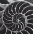
An interesting vector space is the one used in geometrical optics. It allows the treatment of lens combinations in complex systems algebraically without requiring complex ray tracing. The simplest example of this is Gaussian optics. The rays are assumed to remain close to a central axis and stay at small angles to that axis so that the small angle approximation can be used. An "optical bench" with tow lenses and a ray is shown in the figure at the right. The optical axis is drawn as a heavy line. The "ray" is described by giving the height of the ray above (or below) the optical axis and the angle it makes to the horizontal as a function of position. Thus, to describe the ray when it gets to the point s0, we could specify the two numbers h(s0) and θ(s0). We can write these together as a vector:

As the ray propagates through the system, this vector changes. If we keep the angles all small so the small angle approximations hold (sin θ and tan θ ≅ theta), then the propagation of the ray through the system can be described by matrices.

(a) Show that the set of possible ray vectors is a linear space but not an inner product space.

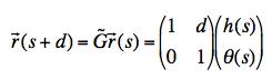
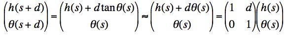
(b) Show that the propagator, that is, the matrix that changes the vector r(s) into the vector r(s+d) when the ray is moving only through empty space is:

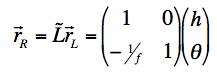
(c) Show that at a thin lens with focal length f the matrix that transforms the ray on the left side of the lens to the refracted ray on the right side of the lens (ignoring the thickness of the lens) is

(Hint: Recall that the focal distance is defined as the point where rays hitting the lens parallel to the axis are bent to cross the axis.)

Solution

(a) The ray vectors can be added and there is a zero vector (the ray parallel to the axis that goes through the center line). There are also inverse vectors (the ray reflected around the center line) so vector addition works. We can multiply a ray vector by any number and there is a "1" and an inverse scalar for every scalar (except 0). The distribution theorems work as we expect so this is a vector space.

We can't really prove that it's not an IP space, but the natural IP that we expect from other examples, namely taking the square of the length of a vector to be the sum of the squares of its components, doesn't work here. You can't add the square of a distance to the square of an angle and get a reasonable result since the dimensions aren't the same.

(b) In order that the vectors/matrices work in a similar way to our figures we'll consider the rays as moving from right to left.

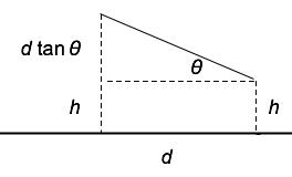
As seen in the figure below, if the ray simply propagates without encountering a lens, it moves along a straight line without changing the angle. In the small angle approximation, the height changes as shown.

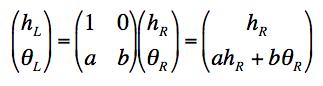
(c) For a thin lens, the height coming in on the right doesn't change as the ray passes through the lens to the left, but the angle does. This means the top row of the matrix has to be (1 0). To see what the bottom row has to be, let's express the ray hitting the lens from the right as (h_R, θ_R) and the ray emerging from the left as (h_L, θ_L). Since we know the height doesn't change, we can assume the matrix has the following form:

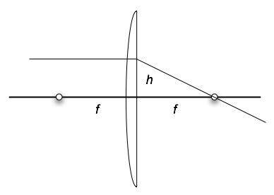
To see what the coefficients a and b have to be, consider two cases. We know from the hint that a ray coming in parallel goes down to the focal point. We also know that a ray coming from the focal point on the right goes out parallel as in the figures below.

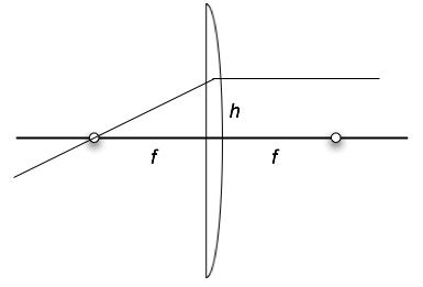
This means that for the left case we have initial values (h,0) going to final values (h, -h/f) where we have used θ ≈ tan θ.

For the right case we have initial values (h, h/f) going to (h, 0). This means we have the matrix equations:

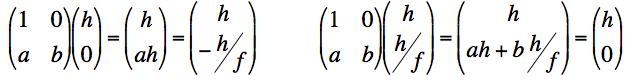
So we can write

ah = -h/f

ah+bh/f = 0

or

a = -1/f

b = 1

as required.

RETURNS

University of Maryland	Physics Department	Physics 374 Home

Last revision 15. November, 2005.