Solving ODEs Numerically

The Half-Step Method

But this doesn't always work. We sometimes find with the Euler method that the errors for each step all have the same sign, adding coherently to produce a much larger error when we are done than we had expected. Taking a smaller step size doesn't reduce our error much because although we cut our error about in 1/2, we add up twice as many of them.

A way of improving beyond the Euler method when this happens is to use a second order method. A clever way of doing this is the half-step method, the simplest one of a collection of higher order approaches known as Runge-Kutta methods.

Example: Newton's Cooling Law

.

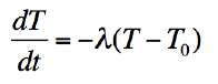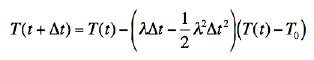
You can, of course, solve this equation for the function T(t) analytically. But let's use it to demonstrate how the half-step method works.

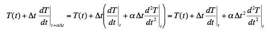
If we use the Taylor series to expand T(t + Δt) about t, we get:

.

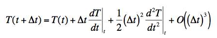In the Euler method, we dropped terms of O((Δt)². Here, we want to keep terms of that order. To do this we use a trick. Note that we carefully specified that all the derivatives in the Taylor series are evaluated at the time t. We want to choose to evaluate the first derivative at a different point -- a point part way to Δt -- and by choosing where we evaluate it, get the effect of the second order term. Here's how that works. If we expand the derivative term in the Taylor series, we get:

.

We want to choose α so that our three-term Taylor series with all the derivatives evaluated at the starting point equals our two term series with the derivative evaluated a part of the way along.

.

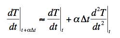
Putting the expansion for the derivative at the shifted point into the equation just above gives:

.

We can easily see that if we take α = 1/2, we will get the Taylor series correct to O((Δt)³).

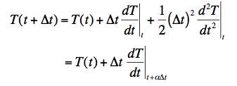
This gives us the following process to generate T(t+Δt):

1. Use the Euler method to calculate T(t+1/2Δt), calculating the derivative at T(t) from the equation.
2. Calculate the derivative at T(t+1/2 Δt) from the equation, using T(t+1/2 Δt).
3. Use an Euler-like step rule to calculate the change from T(t) to T(t+Δt) but using the value of the derivative at the 1/2-step point.

In equations this is just:*

.

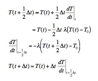Notice that we are not just stepping halfway and then stepping from the halfway point to the end. This would just be the same as making the step half the size. Rather, we are going to the halfway point and calculating the slope there. We then go back to the starting point and make a full-step leap but using the slope we found at the halfway point. Amazingly, this slight of hand results in getting the correct second order stepping rule. (There is a nice geometric interpretation of what's going on here that can be found in many numerical analysis texts.)

Half-Step Method for Newton's Second Law

.

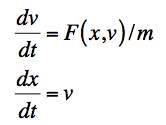We now have two first order equations in two unknowns (x and v) and we can apply the half-step approach to generate a two-step stepping rule.

.

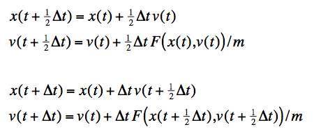Again, notice that we are not just cutting our step-size in half. We are calculating derivatives at the half-step point and then going back to our starting point and leaping a whole step using those derivatives.

* We can just plug these equations into one another to get a single expression for the stepping rule. It is:

.

RETURNS

University of Maryland	Physics Department	Physics 374 Home