Homework Assignments
We will have class in the POWL Lab (room 3115 of the Physics Building) every Friday, and possibly on other dates to be announced as well. Make sure you always bring PC-formatted floppy disks to the Lab (both for classes there and when you are working on assignments there) so that you can save your work. On the first day of class there (Sept. 5) I will provide a floppy disk for each student. There are a large number of demonstration programs available on the server. If you did not get them by downloading the VPython package, you are welcome to copy them to study and to edit to create new programs.
The programming projects and most homework assignments will require creation of computer programs. You can submit the program files from the edit window of IDLE (not the python shell window) in the text of an e-mail. You should check for commands that are more than one line long and insert continuation marks (\) at the end of such lines that are continued on the subsequent line. The files MUST be sent to einstein@wam.umd.edu rather than my usual e-mail address (in which wam is omitted). You will get an automatic reply message that I no longer use this account, but I will for your homework, and the message will serve as your receipt. (Nonetheless, you should always keep a backup copy of anything you submit!!) Your submission MUST have the following format:
1) The subject line on the e-mail is "Phys 165 Set <homework set number>
from <yourname>"
2) The title of the attached file is "<yourname><S#>.py"
3) The listing of the program is pasted into the e-mail
body as text. The first couple lines should contain, as comment statements,
your name and the problem set number.
E.g., "smithS2.py" would be homework assignment two, handed in by student Smith. Finally, it is your responsibility to make sure the file reaches me in a form that works. You should test this in advance by exchanging files with a friend. Failure to follow these directions will result in a major loss of points.
Alternatively, you may copy on onto a PC-formatted floppy disk, and turning in the disk. If I can’t read the disk or open the program files using python, you will again lose many points. So make sure the disk is functioning properly before you hand it in! The disks will be returned to you (with contents) after grading, but, again, you should maintain your own back-up library of disks containing all the programs you have created.
Successful programming requires rigorous logic and considerable organization. To keep your work organized Dr. Williams strongly recommended that you purchase a three ring binder, tabbed dividers, and disk envelopes to use to store all of your course work, class notes, and the documentation that you download. You should also create an annotated index of all the files that you create, and organize the files on your disks with self-evident names in a logical structure of folders. Your python files can also be printed (for storage in your ring binder and easy reading) by copying the text from the IDLE window and pasting it into the editing/word processing program of your choice (e.g. Word, NoteTabLight, bbedit for Mac users, ...) or by using SciTE.
General comment: when turning in homework that involves more than one graphical output, place somewhere between any two the following command
raw_input("Enter a character to continue: ")
For your inspection and information, please find here copies of my routines (modifying EDW routines) for Euler and RK2 integration in a varying gravitational field, in pdf and Winword.
Regarding how to make use of the graphical output window of VPython, note the following info from Windows XP Help:
To copy the window or screen contents Note that this procedure works much better if you set the background color
of the graphic to be white (or a light pastel) rather than black!
To make a copy of the active window, press ALT+PRINT SCREEN.
To copy the entire screen as it appears on your monitor, press PRINT SCREEN.
To paste the image into a document, click the Edit menu in the document window,
and then click Paste.
Set 11: due Wednesday, Dec. 3 or later
This assignment involves learning to use and understand gas.py from the VPython demo package. Since I will not be in shape to lecture much, please spend most of the lab working through the excellent tutorial found at http://wwwmaths.anu.edu.au/comptlsci/Tutorial-Gas/tute-gas.html which describes a very similar program. Note, however, that instead of using uniform, we use random(), which gives a random number between 0 and 1. You can write a simple function for uniform by noting that uniform(m,n) is just m + (n-m)*random(), and uniform(-1,1) is a special case. Students searching for a good topic for the second project might note the suggestions in section 3 of this tutorial!
1. What happens if you substitute xenon (with mass 131 au) for helium (with mass 4 au)? At what temperature would the velocity distribution of xenon atoms be the same as for helium at 300K?
2. Change the way the color is depicted in the graph so that the saturation of the balls decreases (becomes pale and whitish) as the speed increases. Normalize with respect to twice the theoretically-expected average speed. Hints will be provided in class.
3. More to follow, e.g. changing the shape of the box from cubic to rectangular solid.
Set 10: due Wednesday, Nov. 26
Read DEM, chap. 12 (sorry, should have been assigned earlier!)
1. Study the class Point in DEM, chap. 12. Define a class called Polarvector
that creates three-component vectors in spherical-polar coordinates. Your class
should:
a) have attributes r, theta and phi, with theta and phi to be specified in radians
b) allow class objects (instances) to be defined with user-chosen initial values
for r, theta and phi
c) have 4 methods that return respectively the x, y and z components of the
vector, and a three-element list containing the three components
Note that there is an ambiguity in the use of theta and phi! From http://www.physics.orst.edu/bridge/papers/spherical.pdf : "Nearly everybody uses r and theta to denote polar coordinates. Most American calculus texts also utilize theta in spherical coordinates for the angle in the equatorial plane (the azimuth or longitude), phi for the angle from the positive z-axis (the zenith or colatitude), and rho for the radial coordinate. Virtually all other scientists and engineers---as well as mathematicians in many other countries---reverse the roles of theta and phi (and use some other letter, such as R, for the radial coordinate)."
So some math-convention examples are:
http://www.math.montana.edu/frankw/ccp/multiworld/multipleIVP/spherical/body.htm
http://mathforum.org/dr.math/faq/formulas/faq.spherical.html
http://www.geom.uiuc.edu/docs/reference/CRC-formulas/node41.html
http://surendranath.tripod.com/Math/SphCoor.html
While some physics-convention examples are:
http://rkb.home.cern.ch/rkb/AN16pp/node271.html
http://walet.phy.umist.ac.uk/QM/LectureNotes/node62.html
You may use either convention, but please be clear about which you are using!!
2. Define a subclass, Dpolarvector to your class Polarvector. The sub-class will allow you to define theta and phi in degrees. Your definition should introduce new attributes thetad and phid, but allow you to use the original methods of the class Polarvector.
3. (Was 2nd midterm test in 2001, except for minor modifications.) The Lennard-Jones force law, which is similar to the Morse force law discussed in lecture, can be written as:
F_12 = -(12 E/r_eq)[(r_eq/r_12)**13 - (r_eq/r_12)**7](r_12/|r_12|).
This equation gives the vector force acting on atom 1 due to atom 2, where r_12 is the vector pointing from atom one toward atom 2. When r_12 is less than req, the force is repulsive, that is it points in the opposite direction as r_12. When r_12 is greater than req , the force is attractive, that is it points in the same direction as r_12.
For krypton atoms, the value of E is 3.9e-21J, and the value of r_eq is 4.38e-10m.
Write a program to calculate all the pairwise forces acting between a group of krypton atoms, and the net force acting on each atom. Report your forces as vectors, giving the x and y components of each. Apply your program to the specific case of six atoms positioned at:
| atom # --- | x coordinate --- | y coordinate |
| 1 | 0.0 | 0.0 |
| 2 | r_eq | 0.0 |
| 3 | 2 r_eq | 0.0 |
| 4 | 0.5 r_eq | 0.866 r_eq |
| 5 | 1.5 r_eq | 0.866 r_eq |
| 6 | r_eq | 1.732 r_eq |
Here is a useful result to use in debugging your program: For: r_12 = 2 r_eq x, F_12 = 8.2e-13Nx
Prof. Williams's solution is posted here.
4. Dangers of drinking and wandering," adapted from Phys 307 at Syracuse,
offers an engaging application of the ideas of 1D random walk that we have discussed.
You will simulate a drunk person walking back and forth along a straight path.
This path ends at a cliff at which there is no fence. Your goal is to estimate
how likely it is that the person will survive until s/he becomes sober.
a) The assumption is that the person takes random steps back and forth along
a linear path, with the person starting 4 steps away from the cliff edge. That
is, their x-coordinate is initially 0 and if they reach position x = 4, they
plummet to their untimely end. It is dark and they are drunk, so they take a
random step to the left or to the right. Your first step, then, is to decide
how to update the position of the drunk at each time. The probability of going
to the left should be 0.5. If they don't step left, they step right. The size
of the step is 1 at each time. (That is, x is updated to either x - 1 or x +
1, with equal probabilities for each choice.) In other words, you can readily
adapt randomwalk1D.py to do this problem!
b) Set a time counter to zero. The walker takes a step each time interval. At
time 25, the walker sobers up. While [time is less than 25 (they sober up)]
AND [x<4 (they are still alive)] have them take a random step. If they plummet
during this time, i.e., they reach x = 4, count a "fatality". If they
don't fall off within 25 steps, they sober up "survive". For your
simulation, you might have the walker take 10 steps a second or so, so that
it doesn't take forever to run, but slow enough that you can see the motion.
c) Repeat the trial, that is, step (b), a large number of times. After each
trial, regardless of whether the walker survives, set the walker back at the
origin to try again.
d) You can draw the walker as a sphere. (At your option, if you like
working with frames, you can make the animation more interesting by depicting
the walker as a frame object in which you attach a cylinder and a sphere (or
more) to make a person. You would then change the pos attribute of the frame
to make the person move.) Mark the cliff edge somehow (with a cone? a curve?
whatever you choose.)
e) Redo the problem assuming there is a weak wind blowing to the right, so that
the walker is 10% more likely to go to the right than to the left. (Thus, you
will need to change the inequality for p.)
Submit a working revision of the program and your estimates of the survival
probability without and with wind.
Set 9: due Friday, Nov. 14
Read DEM, chaps. 13, 14; also Zelle (online; see class URLs), chap. 10, sections 1-4
1. Exceptions: Write a short program to input two numbers from a file,
divide the first number by the second, and output the result to the screen.
Include an error-handling sequence to catch (and print appropriate messages
for) three types of errors:
a) an I/O error if the file cannot be opened
b) a value error if the input values can't be converted to a numeric type
c) a divide-by-zero error.
See section 2.3 of the Python Library Reference for the names of exception and section 8.3 of the Python tutorial or section 11.5 of DEM for examples.
The following problems are adapted from Lab 9 of Phys 307 at Syracuse U. in Fall 2002
2. Review of recursion (cf. DEM sections 4.9 and 5.5). In the simplest form of recursion, a function calls itself. The function solves a problem or carries out a procedure that is defined using, in part, itself. E.g., suppose you want to sum all of the numbers from 1 to n. Let S(n) be this sum. The value for n=1 is simple: S(n)=1. When n>1, S(n-1) is the sum of the numbers from 1 to n-1, so that S(n)=S(n-1)+n.
Translate this idea into a computer program in python. Write a function isum_up_to(n)
defined using a def statement. In this function, use an if statement to determine
what value to return: if the argument n is equal to 1, return the sum of the
numbers up to 1, that is, 1. If the argument is greater than 1, return n plus
the sum up to n-1. Use this function and check the output values for a couple
of values of n. Include your code in your submission.
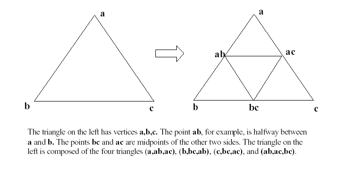
3. In this problem we create an object with a non-integer (fractal) dimensionality. This so-called Sierpinski gasket is made out of a sequence of triangles in a well-defined procedure. While drawing the objects, we will keep track of the number of triangles used, in order to compute the fractal dimension. The basic idea is to draw an equilateral triangle, divide it into 4 equilateral subtriangles as in the sketch below, and then remove the central (downward-pointing) triangle. Next, on each of the 3 remaining triangles, we do the same procedure: divide into 4 subtriangles and remove the central one.
a) First we try just subdividing the triangle without removing the central subtriangle:
the following program will divide a triangle into subtriangles n times, to draw the original triangle:
from visual import *
def tri(a, b, c, level):
if (level == 0): ## smallest subtriangle
convex(pos=[a,b,c]) ## draws an object that contains 3 pointselse: ## find midpoints, delegate to next level
numtriangles = 1
ab = (a+b)/2numtriangles = tri(a,ab,ac, level-1) + tri(b,ab,bc, level-1) \
ac = (a+c)/2
bc = (b+c)/2
+ tri(c,ac,bc, level-1)+ tri(ab,ac,bc, level-1)
return numtriangles ## The function returns the total number of triangles drawn.
## use the function
n=5
m = tri(vector(-1,-.5,0), vector(0,1,0), vector(1,-.5,0), n)
print m,"triangles at level", n, "at length scale",(1/2.)**n
Run this program for values of n up to 7 and plot the relationship between length
scale and the number of triangles. This sequence of objects has integer dimension
(area proportional to [linear dimension]**2).
b) To produce the Sierpinski gasket, remove the central triangle from the statement giving numtriangles. What is the slope of the number of triangles vs. the size of the triangle (the level)? Note that the fractal dimension df is log3/log2 = 1.585...(that is, area proportional to [linear dimension]**df).
c-OPTIONAL) Save your code to a new file pyramid.py.
i) Modify the tri function to take 5 arguments: a, b, c, d, and level.
ii) Under the if statement, draw a convex object that includes a, b, c, and d. (Just add d to the list of points in the pos argument.)
iii) Under the else statement, comput new midpoints ad, bd, and cd.
iv) Then draw 4 tetrahedra (a,ab,ac,ad) etc., and find the fractal dimension, showing it is less than 3.
4. In VPython, the frame object can be used to group objects into a single object. frames have pos and axis attributes that give their orientation to the frame in which they are defined. Rotations and translations of the frame move the associated objects as a rigid object. This is programmed by (a) creating a frame using the frame() function and (b) assigning or attaching objects to the frame, for example, when they are created. What you learn about frames here will be used to study more natural looking fractals next week.
For example, the following creates a frame f and associates a sphere and a cube with that frame:
from visual import *
scene.autoscale = 0
f = frame()
cylinder(frame = f, radius=0.3, pos = (-2,0,0), axis=(4,0,0), color=color.yellow)
sphere(frame = f, pos=(-2,0,0), color=color.red)
sphere(frame = f, pos=(2,0,0), color=color.red)
Check that when you run this, nothing spectacular happens (frames are invisible.) But now add this loop to the above:
while 1:
rate(40)
f.rotate(angle=0.05, axis=(0,0,1))
f.pos = f.pos + vector(0.01,0.01,0)
and note what happens!
You can also chain frames together: a frame can belong to a frame. You can make lists of frames. Note this about lists: you can refer to a member of a list by giving its position in the list: the first item is at position [0], the second item is at position [1], the third item is at position [2], etc. Negative numbers count from the end: position [-1] gives the last item in the list, position [-2] is next to last, etc. Try out the following examples:
alist = [5, 9, 43, 27,25]
print alist[0]
print alist[1]
print alist[4]
print alist[-1]
from visual import *
boxlist = [box(), box(pos=(1,1,1)), box(pos=(3,3,3))]
boxlist[1].rotate(angle = 2, axis=(0,0,1))
Now use frames and lists together. Make a program by
a. importing visual.
b. turning off scene.autoscale
c. starting a list named framelist with a single frame (default values).
d. Check that your program works so far. Note that frames are invisible and
you are simply seeing that you have made no errors so far.
e. start a for loop - step through the numbers from 0 to 15. In this
loop:
i) set prev_frame to be the last item of framelist. Run your program
to make sure there is no error.
ii) create new_frame, a frame that is a subframe of prev_frame
(that is, frame = prev_frame should be an argument to the frame() function),
has an axis attribute of (0.9,0.,0.1), and a pos attribute of (0, 0.5, 0). Run
your program again.
iii) append new_frame to framelist. Run your program again.
iv) create a box that has new_frame as its frame and has a height of
0.2.
Set 8: due Friday, Nov. 7
This is a minimal assignment, since at least a third of the class is either sick or involved with physics meetings, and since many of you still have lots to do on the midterm project. I remind you that I want something turned in on Nov. 7, even if it is not all you had proposed to do in your earlier submission. Note that I will be at a meeting in Baltimore much of next week, and so am canceling class on Wednesday, Nov. 5, to be rescheduled once we regroup.
1. Download soundspeed.py , which we have analyzed in class. Implement each of the two ways to compute the speed of sound and compare the results. (Cut and paste your output into what you submit.)
2. Download crystal1D.py, extract the graphics part, and combine it with soundspeed to display the motion of the atoms as the pulse moves down the chain instead of the existing graphs of the displacements of atoms 0 and 15. In order to see the displacements, you should enhance them by a factor of 5 (for the graph only, not for the actual displacements in the Euler integration). [So plot i*req + 5.*(xlist[i]-i*req).] Note that you will need only a very small part of crystal1D.py: just the parts that do the drawing using the VPython sphere object, the color setting, and makespring if you want springs, and something to generate the list of "pos" values for the graphic. You do not need the many attributes of a, nor the parameters for the chain, nor the momentum or evolution parts. You certainly do not want the random number generation of velocities! Hope crystal1D.py is more helpful than problematic!
SOLUTION NOW DOWNLOADABLE here
Extra things to do, for those with time to spare (i.e. not mandatory):
1. Extend the time range of soundspeed so that the pulse returns to the origin. See whether the speed of sound is consistent with what you found above, and find the maximum displacement of the 0th atom. Compare that with the initial displacement of req/10. Note that to do this, you will need to set up a variable that stores the maximum placement of the 0th atom (comparing it to the displacement at any instant during the evolution and updating when needed), but you must be careful not to start this process until the initial pulse has moved far away from the 0th atom!
2. Play with the colors in crystal1D.py so that something changes (e.g. saturation or value/intensity) as the atoms displace from their equilibrium positions.
3. Modify the display in either crystal1D.py or its graphics as applied to soundspeed so that displacements are shown in the vertical direction (moving up or down from the equilibrium position) rather than the horizontal direction.
Set 7: due Wednesday, Oct. 29
1. Most of this exercise is to gain better understanding of how setting color with RGB works. Type in the following short code, which generates a spiral that evolves from magenta (1 0 1) at time 0 to cyan (0 1 1) at the end, time 10. Be sure to rotate your field of view out of the x-y plane (drag with your mouse while right-clicking) to get a 3D view.
from visual import *
helixcurve = curve(radius=0.05)
for t in arange(0,10,0.01):
rate(100)
helixcurve.append(pos=(cos(3*t),sin(3*t),t), color=(1-t/10., t/10., 1))
Note that the code could also have been written
from visual import *
helixcurve = curve(radius=0.05)
for t in arange(0,10,0.01):
rate(100)
helixpointcolor=(1-t/10., t/10., 1)
helixpos=(cos(3*t),sin(3*t),t)
helixcurve.append(pos=helixpos, color=helixpointcolor)
a) Modify the code so that the spiral evolves from yellow to blue: you need only change the argument of color=( ), or the right side of helixpointcolor=( ) in the alternative code.
b) Modify the code so that the spiral is white in the first quadrant (x>=0,y>=0), blue in the second quadrant (x<0,y>=0), green in the third quadrant (x<0,y<0), and red in the fourth quadrant (x>=0,y<0). It is simplest to use if, else, and perhaps elif statements to do this. Students seeking a challenge can then try setting the color using a Boolean-like function (that checks whether the argument, in this case x or y, is >= or < 0 and returns 1 or 0; cf. DEM, Section 5.4) or Boolean variables to express whether x and y are positive [actually, non-negative] or negative [e.g ixneg=(x<0), which is 1 if x is negative and 0 otherwise]. [Warning: Python 2.3, unlike versions 2.2 and earlier, admits a Boolean type with values True and False rather than 1 and 0, but this does not seem to be a problem in the present context.]
What happens if you change sin(3*t) to -sin(3*t)? [This was originally the
third part, but it seems "off-message".]
2. There are two modules, written by Prof. A. Middleton, available from the Syracuse University Physics 307 web repository; then click on Assignments, then Lab#7, part 2. If you pick the .doc version, you can cut-and-paste the programs. Save these modules as gravityAM.py and fakesolarsystemAM.py on your computer.
gravityAM.py defines the forces of gravity and updates the position and curve that records the path of a planet. There are two functions defined in it. The function gravaccel computes the acceleration due to gravity on a planet at a given position due to a planet having another position and mass. The function update updates the position of a planet based upon its velocity. This function also updates the velocity by adding up [vectorially] all of the acceleration vectors that act on the planet. It tracks the position of the planet by appending points to the curve associated with the planet, at the position of the planet.
fakesolarsystemAM.py gives coordinates, velocities, masses, and visible sizes to the Sun, the Earth, and to Mars. Mars's position and velocity are not quite accurate, and and as part of this assignment you will vary its mass.
Investigate the dynamics of a solar system that resembles ours. The fakesolarsystem.py
module has zero mass for Mars, which is approximately true as far as the Earth
is concerned. To get the simulation started, you need to write a program, saved
as theplanets.py. This program will need to:
a) Import the functions defined gravity.py and make use of (by cut-and-paste)
the code in fakesolarsystem.py.
b) Set scene.autoscale to 0.
c) Have a while 1: loop that, at a particular rate, executes the function update
for all of the objects in the list planets.
Execute this program and observe the results.
3. Increase the mass of Mars to 0.02. (This mass is in units of solar masses:
the Sun has a mass of 1.0.) Repeat your simulation. NOTE: whenever you modify
fakesolarsystem.py, make sure to save it so that your program theplanets.py
will load the updated module. Finally, try a mass of 0.05. In the Syracuse version
you are asked make the mass of Mars sufficiently large to induce chaotic behavior
in Earth's orbit.
Set 6: due Wednesday, Oct. 22
Read DEM, chaps. 10, 11
1. a) Write a program, using VPython, to display a set of N spheres
of radius 0.5 equally spaced around the circumference of a circle of radius
R . The program should be able to read in the values of N and R from the screen
(although this flexibility should be added only after doing the rest of the
problem). The coordinates should be calculated and stored in a list using a
For command.
The program should output this list of x-y coordinates to the output window
and display the spheres on a visual display screen.
b) Write a function to draw a cylinder (visual graphic object) between two spheres. The input to the function will be the spheres’ positions, radii, and color. You should make the cylinder’s position such that it appears to connect the two spheres, and you should make the cylinder’s radius half that of the spheres and color different from that of the spheres.
c) Have the program in part a) use the function of part b) to create
a circular "necklace" of spheres connected by cylinders.
2. Use orbits.py or my modification of it to find a) the ratio of the largest distance between the orbiting stars and the smallest distance between them, and b) the value of initial momentum that produces circular orbits. (HInt: what is the relationship between velocity and acceleration for an object undergoing uniform circular motion?)
3. Go through the documentation of rattrap.py , in which the program is in FORTRAN 4 but has been translated here. Note the flowchart. Figure out why the python program does not print the last line, and fix it.
Note that on Oct. 24 you need not hand in the completed midterm project but must submit a progress report including a flow chart (and/or detailed prose description of the program you are writing) and the program that you have written to date, with clear documentation. The final project submission will be due about 10 days later, depending on when I can get your progress reports returned (so about a week after that return date).
Set 5: due Tuesday, Oct. 7
Read DEM, chaps. 9, 10.
1. Write a program that produces a histogram with 10 equally-spaced bins for 100 random numbers. You may find it convenient to start with the function randomList in section 9.5 of DEM. Then generalize, for the version you turn in, to allow the user to enter (interactively) the number of random numbers to be generated and plotted in the histogram. You will need to look someplace besides DEM for this, e.g. Gauld, chap. 10 or Zelle, section 2.5.2: the form is
integerToBeUsedInProgram = input("Enter the number of random numbers to use: ")
2. To polish off the study of errors on set 4, plot the error vs. increment size for the Euler runs and for the RK2 (2nd order Runge-Kutta) runs. On the horizontal axis should be the power of sqrt(10) by which you divided dt (i.e., essentially the logarithm of the time interval). On the vertical axis should be the logarithm of the difference between the final computed value of the velocity and the analytically-predicted value. (To restate this, plot pairs of points given by the power of sqrt(10) and the log10 of the velocity "discrepancy" for that run.) It should be easy to collect these points from the runs in set 4, preferrably using the computer but if necessary by hand. The goal is to see whether these points lie on a straight line, characteristic of power-law convergence with decreasing dt.
3. Redo/do problems on set 4 that you got wrong or could not turn in o, which evidently is giving lots of difficulties.
Set 4: due Wednesday, Oct. 1 -> Friday, Oct. 3; bonus for submission on original date
Read Downey et al. [hereafter DEM, no offense intended to classmembers who are Republicans], rest of chap. 8
Read Numerical Python (see class URLs): chap. 5 on Array Basics and chap. 8 on Array Functions. In particular, learn about take, put, transpose, diagonal, trace, sort, searchsorted, concatenate, inner product, resize, and identity.
1. Do parts b), c), and d) of set 3. Include a plot of the velocity vs. time (plus any other plots you care to add), and a line indicating the predicted (based on conservation of energy) velocity of the dropped mass on impact with the earth.
2. Write a Python program that a) plots as a smooth curve, for x between -pi and pi, a) the simple function cos(x) and b) the function cos(x)/(x-pi/2.). Label the axes and supply a title for each graph. Note that you will need to devise a way to deal with the form 0/0 at x = pi/2. (Before writing the program for part b, use L'Hopital's rule to find the value at this point.)
3. For even integers n between 10 and 100:
a) create a list g(n) = ((n - 1) times the logarithm of n in base 10) for n <= 50, and g(n) = g(n=50) divided by the hyperbolic cosine of (n/25 -1) for n > 50.
b) draw a graph of g(n) vs. n (using gdots).
c) create a list of the values of g(n), sorted in ascending order.
d) create a histogram of the values of g(n) over the given range, using about a half dozen bins (of equal width).
e) [optional challenge!!] devise an elegant way using features of NimPy to arrange the pairs [n, g(n)] in ascending order of g(n).
4. Skim through one of the online references, focus on the material we have covered so far in Phys 165, and comment in a paragraph or two how the treatment compares with that in DEM.
Set 3: due Friday, Sept. 26 (problem 2 plus just part a) of problem 1--the later parts are postponed---please let me know if hurricane-related power outages hinder your ability to do this assignment punctually
Read Downey et al., chaps. 6, 7
Study Graph Plotting section of VPython manual
Study Euler and related methods of numerical integration in the references on the class listing. Also I will pass out a few pages from the CUPS book on Classical Mechanics. For those with good preparation, take a look at the standard reference, Numerical Recipes (online or printed), sections 16.0, 16.1, 16.5.
1. To do a good study of simple routines for numerical integration of second-order differential equations, in particular Newton's equations, we need a force which depends at least on position. Hence, we need something more sophisticated than bounce.py. Instead, we will start with a program from the previous offering of Phys165, looking at falling in the earth's gravitational field over distances that are not small compared to the earth's radius Re. In class we will try some modifications to this program. Then you will check the dependence of errors on the time-step size dt.
a) Start with dt = 100 sec., then decrease by a factor of about sqrt(10) so that every second run involves dt being an integer power of 10) until you achieve convergence (in the sense that the final velocity does not change by more than 0.1%).
Then try again with various more sophisticated integration schemes:
b) Average the "old" and "new" velocity, as at the end of the Chabay & Sherwood handout.
c) Do the second-order Runge-Kutta method, as in eq. 2.14 of the CUPS handout.
d) For extra credit, if you have time and energy, do the fourth-order Runge-Kutta method. (The relevant equations are given on the homework handout.
2. Use the various list operations to do the following exercises. As part of each of the "create" task, print it with a print statement tahat includes an appropriate description.
a) Create a list ia1 of odd integers between 0 and 20, using a single command.
b) Produce a graph of these cubed integers (plotted vs. integer) using gdots from visual.graph.
c) Create another list ia2 of the cubes of these integers.
d) Create as ia3 a list in which you delete 9 and 11 from ia1, using a slice command.
e) Create as ia4, containing the same elements as ia1 but in reverse order.
f) Create as ia5 a list with the elements of ia3 in ascending (smallest-to-largest) order followed by the same elements in descending order.
g) Create as ia6 the elements of ia5 sorted in descending order.
h) Find the number of elements in ia6.
Set 2: due Monday, Sept. 15
Read Downey et al., chaps. 3, 4, 5, 8.1-8.3,8.6-8.7
Programming problems:
1. Given the vertices of a triangle as input variables, find the area of the triangle. You will find the math functions of the visual module to be of use. For simplicity, take one vertex at the origin, the second somewhere along the (positive) x-axis, and the third anywhere in the first quadrant. (So there are 3 variables to input. Assume the units to be meters.)
a) Find the area straightforwardly by computing half the base times the height. Print this result as output with an appropriate description.
b) Recompute and print out (with appropriate prose) the area of the triangle using Heron's Formula: area = sqrt[s*(s-a)*(s-b)*(s-c)], where s=(a+b+c)/2 and a, b, c are the lengths of the 3 sides of the triangle. Check that the results in parts a and b agree! The program you submit should contain both methods of computation of the area of the triangle (and the print statements to output the results) and be labelled trianglearea.py.
2. Modify bounce.py to describe a projectile that is a) launched horizontally (in the positive x direction) rather than vertically, b) on the moon (where g=1.6 m/s**2) and c) stops when it hits the ground, rather than bouncing. (Hint: you might find the command break to be convenient, though it is by no means necessary to do this exercise easily. The effect of break is to stop iterations in a loop. d) Decrease the size of the ball from its default value of 1 [m] to 0.25 m and find (by trial and error) the largest initial horizontal velocity (to 1 decimal place in m/s) such that the ball on the moon still strikes the horizontal plate. Submit the program that you use to do part d), labelling it bouncemoon.py.
HInts:
It is often easier to write programs with sample values of the input parameters specified internally, rather than via input dialogs, so that the test program will run without interuption for input. Once operational, the input statement[s] can easily be substituted for the internal initialization.
The simplest python input statement for importing numbers has the form:
xval = input("Enter the value of xval: ")
Note the useful command break to escape from a loop, mentioned above.
Reminder of the steps in software development:
1) Specify the problem requirements
2) Analyze the problem, determining inputs, outputs, and production formulas relating them
3) Design the algorithm
4) Implement (program) the algorithm
5) Test and verify the program
6) Document the program for future use
Set 1: due Monday, Sept. 8
Read Downey et al., chaps. 1, 2
Read Gauld, chap. 5 or sidebar on Simple Sequences at http://www.freenetpages.co.uk/hp/alan.gauld/
Skim the VPython reference manual, found at http://www.vpython.org/webdoc/visual/index.html . You should have this file readily available to you at all times, either by printing it out or/and by loading the html files onto the computer you routinely use. You can download a zipped file of the html, named Doc-2003-08-09.zip , from http://www.vpython.org/all_download.html . (Note that my Word document self-destructed ("repaired itself").)
Exercises:
1. a) Print a simple greeting, like "Hello, World!" Note that Python is case-sensitive: you must write print, not Print or PRINT ! Try using double quotes, single quotes, and pairs of double quotes.
b) Now include an explanatory comment (using #) on the same line of input.
2. Use Python as a calculator to:
a) Add 2 numbers.
b) Multiply 2 numbers.
c) Compute a complicated expression involving addition, multiplication, subtraction, and parentheses.
d) Exponentiate (**), e.g. find 2 raised to a large power.
e) Provide an illustration of the difference between integer and real[-number] division (/). This is less intuitively obvious than the previous. Note that % is the mod or modulus (or remainder, in elementary school parlance) operator; illustrate how it works.
3. Explore specifying numbers in strings in Python using % markers. (This is another use of %, different from the mod operator. There should be no confusion.
%d: integer
%f: real
%s: string
%x: hexadecimal
a) Rewrite some of your calculator problems above, e.g.
>>>print "The sum of %d and %d is %d" % (17, 28, 17+28)
b) Now explore specifying the format.
E.g. %0.2f is a real number with 2 decimal places, possibly 0's. (You could also write %.2f)
%04d is an integer padded to 4 digits by adding 0's in front.
%4d is an integer padded to 4 places by adding blank spaces in front.
%9.2f is a real number with 2 decimal places, taking up 9 spaces in all, counting the decimal point: so 6 spaces before the decimal point, filled with blanks if the number is not large enough.